Unizor is a site where students can learn the high school math (and in the future some other subjects) in a thorough and rigorous way. It allows parents to enroll their children in educational programs and to control the learning process.
Euler-Lagrange Equations
for the Gravitational Field
The following is an illustration of using Lagrangian Mechanics to analyze the movement of a planet in a central gravitational field of the Sun.
It will also show how the Kepler's laws of planetary movements are derived from Euler-Lagrange equations.
Let the Sun be modeled as a point mass M and a planet be modeled as a point mass m.
In the lecture about a central field we proved that the orbit of a planet lies in a plane. That allows us to choose polar coordinates r(t) and θ(t) with the Sun at the origin as generalized coordinates.
To apply Euler-Lagrange equation, we have to express kinetic energy T and potential energy U in terms of generalized coordinates r and θ.
Kinetic energy depends on the square of the magnitude of velocity v. In polar coordinates this is expressed as a sum of squares of radial speed vr and perpendicular to it tangential speed vθ: vr = r' vθ = r·θ' v² = vr²+vθ² = (r')²+(r·θ')² T = ½mv² = ½m[(r')²+(r·θ')²]
Potential energy of a planet in the gravitational field (you can refer to lectures in Physics 4 Teens → Energy → Energy of Gravitational Field) is U = −G·M·m/r
where G is the universal Gravitational Constant
Lagrangian of a planet is L = T − U =
= ½m[(r')²+(r·θ')²] + G·M·m/r
The Euler-Lagrange equations for generalized coordinate are ∂L/∂r = d/dt ∂L/∂r' ∂L/∂θ = d/dt ∂L/∂θ'
From the equation for r: ∂L/∂r = m·r·(θ')² − G·M·m/r² ∂L/∂r' = m·r' d/dt ∂L/∂r' = m·r"
Resulting equation is m·r·(θ')² − G·M·m/r² = m·r"
Cancelling m produces r·(θ')² − G·M/r² = r"
From the equation for θ: ∂L/∂θ = 0
(because L does not explicitly depend on θ) ∂L/∂θ' = m·r²·θ'
Resulting equation is 0 = d/dt m·r²·θ'
from which follows that m·r²·θ' = const = |L|
The expression on the left side of the above equation is the magnitude of a angular momentum vector (usually it's denoted by symbol L, but we will use |L| to separate it from the Lagrangian).
Since the Lagrangian does not depend explicitly on θ, this coordinate is cyclic, and therefore the corresponding angular momentum is conserved.
So, this equation expresses the angular momentum conservation law.
At the same time the constancy of the expression r²·θ' means that equal areas are swept by the radius vector per unit of time. Thus, Kepler's Second Law follows directly from the Euler–Lagrange equations.
From this follows that r²·θ' is also a constant of motion (angular momentum per unit of mass), let's call this constant k. Now the second Euler-Lagrange equation looks like this r²·θ' = |L|/m = k
The system of both Euler-Lagrange equations for two generalized coordinates is
r·(θ')² − G·M/r² = r" r²·θ' = k
From the physical standpoint, the second equation determines how fast the planet moves along the orbit, while the first determines the shape of the orbit.
Let's use the expression for θ'=k/r² from the second Euler-Lagrange equation and substitute it into the first term r·(θ')² of the first equation r·(θ')² = r·(k/r²)² = k²/r³
Now the first equation looks like k²/r³ − G·M/r² = r"
This is exactly the equation we derived in the lecture Motion in Polar Coordinates of the Laws of Kepler part of this course, though the derivation in that part was much longer and involved a lot of vector manipulations in Cartesian coordinates.
Both Euler-Lagrange equations define r(t) and θ(t) as functions of time.
In a tradition of using polar coordinates, let's derive r as a function of θ.
Differentiation by time of an expression X can be done according to the following procedure
[A1] dX/dt = (dX/dθ)·(dθ/dt)
or, equivalently,
[A2] dX/dθ = (dX/dt)/(dθ/dt) = X'/θ'
Apply rule [A2] for X=r: dr/dθ = r'/θ'
and, therefore,
⇒ r' = (dr/dθ)·θ' =
use the second Euler-Lagrange equation above resolving it for θ'=k/r²
= (dr/dθ)·k/r² = −k·d(1/r)/dθ
Consider the equality we've got r' = −k·d(1/r)/dθ
Let's differentiate it by time. On the left side we will get r".
To differentiate d(1/r)/dθ on the right side by time, we will use the rule [A1] above getting d/dt[d(1/r)/dθ] =
= d/dθ[d(1/r)/dθ]·(dθ/dt) =
= [d²(1/r)/dθ²]·θ' =
= [d²(1/r)/dθ²]·k/r²
Equating derivatives of the left and the right sides, we get r" = −(k²/r²)·[d²(1/r)/dθ²]
This expression for r" we substitute as the right side of the first Euler-Lagrange equation getting r·(θ')² − G·M/r² =
= −(k²/r²)·[d²(1/r)/dθ²]
Multiplying both sides by r²: r³·(θ')² − G·M =
= −k²·[d²(1/r)/dθ²]
Again substitute θ'=k/r² getting r³·k²/r4 − G·M =
= −k²·[d²(1/r)/dθ²]
or (1/r) − G·M/k² = −[d²(1/r)/dθ²]
Assign x=1/r. In terms of x as a function of θ our equation becomes d²x/dθ² + x = G·M/k²
This is a known type of differential equation, in a simplified form its solutions are x(θ) = a + b·cos(θ)
More precisely, the general solution is x(θ) = G·M/k² + C·cos(θ−θ0)
from which follows r(θ) = 1/[G·M/k²+C·cos(θ−θ0)]
The last equation in polar coordinates represents second degree curves (called conic sections - circle, ellipse, parabola, hyperbola) with eccentricitye=C·k²/(G·M).
Geometrically,
if e is smaller than 1, a curve is an ellipse;
if e is equal to 1, a curve is a parabola;
if e is greater than 1, a curve is a hyperbola.
This equation describes an orbit of an object flying around the Sun along a trajectory that is a conic section. This is in compliance with Kepler's laws of planetary movement.
Thus, using the methodology of Lagrangian Mechanics, we were able to derive the Law of Conservation of Angular Momentum, Kepler's Second Law and the shape of a planetary orbit - a curve of the second degree (conic section).
As we have learned by now, Euler-Lagrange equations in Cartesian coordinates are equivalent to Newton's Second Law, provided the forces are derivable from a potential and constraints are ideal (do no virtual work).
At the same time Euler-Lagrange equations are applicable not only in Cartesian coordinates, but in generalized as well.
In simple cases of conservative mechanical systems in Cartesian coordinates Newton's Second law might be even a preferable choice, but in complex cases of multiple objects moving and acting upon each other the complication of using vectors of force and acceleration might prompt us to choose Euler-Lagrange equations in Cartesian or generalized coordinates as the main tool to obtain trajectories of moving objects.
There is, however, another reason why Euler-Lagrange equations might be a better choice.
In previous lectures we discussed a few times a simple case of a pendulum in a gravitational field.
The specifics of this example is that the movement of a pendulum is constrained by a rigid rod, which necessitates introduction of constraints into a system of equations based on the Newton's Second law.
In the lecture Pendulum of this chapter we approached the task of finding the formula of this pendulum's movement using an angle of deviation of its rod from a vertical. We started analyzing the problem using Cartesian coordinates, but gave up noting the complexity of the problem.
This was not really the application of Newton's Second law. Actually, we used the non-Cartesian parameter (angle) to solve the problem, and we expressed the movement in terms of this angle, not the Cartesian coordinates of the pendulum's bob.
Let's try to move with Cartesian coordinates a little further to make sure that this is not a good way to approach this problem.
Here is how this task is supposed to be approached using the classical Newtonian approach.
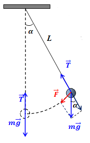
Let x(t) and y(t) be time-dependent coordinates of a point-mass bob at the end of a rod moving along a circular trajectory. Assume, positive direction of the X-axis on a picture above goes to the right and positive direction of the Y-axis goes down.
Then an angle α of a deviation of a rod from a vertical is defined by cos(α(t)) = y(t)/L sin(α(t)) = x(t)/L
Two forces act on a bob of a pendulum:
(a) constant weight W directed vertically down along Y-axis, its projections on coordinate axes are: Wx = 0 Wy = m·g
(b) tension of a rod T(t) that holds the bob on its end, its unknown magnitude is T(t) and its projections on coordinate axes are: Tx(t) = −T(t)·sin(α) = −T·(x/L) Ty(t) = −T(t)·cos(α) = −T·(y/L)
These parameters allow to construct differential equations of motion based on Newton's Second law m·x"(t) = −T(t)·(x/L) m·y"(t) = m·g − T(t)·(y/L)
In addition, we have to satisfy the constraint x²(t) + y²(t) = L²
We have three equations with three unknowns x(t), y(t) and T(t).
We will skip (t) for brevity.
First, let's eliminate T by invariant transformations of the above equations.
(a) transfer m·g in the second equation to the left m·x" = −T·(x/L) m·y" − m·g = −T·(y/L)
(b) multiply the first equation by x, the second - by y and add them together m·x·x" + m·y·y" − m·y·g =
= −T·(x²+y²)/L
(c) note that x²(t)+y²(t)=L², which allows to substitute it into the above equation and resolve it for T m·x·x" + m·y·y" − m·y·g =
= −T·L T = −(m/L)·(x·x" + y·y" − y·g)
(d) by differentiating an identity x²+y²=L² by time twice we get another identity: 2x·x' + 2y·y' = 0 x·x' + y·y' = 0 x'² + x·x" + y'² + y·y" = 0 x·x" + y·y" = −(x'² + y'²)
(e) use this in the expression for T above T = (m/L)·(x'² + y'² + y·g)
(f) we can substitute T with its expression from (e) into original equations getting two equations with only two unknown functions x(t) and y(t) (mass m cancels out) x"(t) = −(x/L²)·(x'²+y'²+y·g) y"(t) = g−(y/L²)·(x'²+y'²+y·g)
The solution to the above system of differential equations is lengthy, it does not resolve into any elementary functions and the obtained integral as a solution is not pretty (it involves elliptical functions).
Let's forget about Cartesian coordinates and switch back to an angle as the main parameter.
It has two main advantages:
(a) there is only one parameter, not two like in Cartesian coordinates;
(b) there is no need to involve a constraint because it is implicitly built into an approach we took.
In the simplest form for the above example, two Cartesian parameters (x and y) minus one constraint (x²(t)+y²(t)=L²) results in one unconstrained parameter (angle α in this case) that is one degree of freedom.
The above can be generalized to the following.
Consider a mechanical system moving in n-dimensional configuration space and described by n time-dependent coordinates: s1,...,sn.
Assume, there are m constraints that affect the motion of this system f(1)(s1,...,sn)=0,
...
f(m)(s1,...,sn)=0.
Then under certain conditions (see below) the movement of this system can be described by n−m generalized parameters, which means that the system has n−m degrees of freedom.
These conditions include:
(a) constraints must be holonomic (expressed as equations that contain functions of only coordinates and time, not the velocities or other non-positional parameters);
(b) constraints must be independent (not derived from one another) which for holonomic constraints would follow from the requirement of linear independency of their gradients.
It should be noted that each individual constraint, provided its gradient is nonzero, defines a surface (a smooth manifold of dimension n−1) in a configuration space.
A trajectory of a system constrained by m holonomic constraints with linearly independent gradients belongs to an intersection of all such surfaces (which is a smooth manifold of dimension n−m) defined by all m constraints.
The system's velocity at any point on its trajectory must be tangential to this intersection of surfaces and, therefore, perpendicular to each constraint's gradient.
With m linearly independent gradients that together span an m-dimensional space, the tangent space where all trajectories belong to span orthogonal to it (n−m)-dimensional manifold, and generalized coordinates are just coordinates in this constrained manifold.
The rigorous mathematical proof of the above statement and exact specification of conditions of its applicability are beyond the scope if this course.
However, some geometric interpretation might be helpful.
Imagine the n-dimensional Euclidean space Rn and a single constraint in it f(s1,...,sn) = 0
For example, for a movement of a single point-mass we use n=3, our own three-dimensional space R3 with Cartesian coordinates x, y and z in it and a constraint - an equation of a sphere of radius r x²+y²+z²=r².
The constraint means that the movement of our mechanical system expressed as coordinate functions of time si(t) (i∈[1,n]) is such that f(s1(t),...,sn(t)) = 0
for any moment of time t.
In our example it means that a point-mass must be always on a surface of a sphere, which can be parameterized by only two parameters.
In general, under conditions described above, one constraint reduces the number of degrees of freedom of a mechanical system by one.
Notes to a video lecture on http://www.unizor.com
Transverse Wave
We are familiar with longitudinal waves, like sound waves in the air.
Their defining characteristic is that molecules of air (the medium) are oscillating along the direction of the wave propagation, which, in turn, causing oscillation of pressure at any point along the direction of wave propagation.
Consider a different type of waves.
Take a long rope by one end, stretching its length on the floor. Make a quick up and down movement of the rope's end that you hold.
The result will be a wave propagating along the rope, but the elements of rope will move up and down, perpendicularly to the direction of waves propagation.
(open this picture in a new tab of your browser by clicking the right button of a mouse to better see details)
These waves, when the elements of medium (a rope in our example) are moving perpendicularly to a direction of waves propagation, are called transverse.
Such elementary characteristics of transverse waves as crest, trough, wavelength and amplitude are clearly defined on the picture above.
Some other examples of transverse waves are strings of violin or any other string musical instrument.
Interesting waves are those on the surface of water. They seem to be transverse, but, actually, the movement of water molecules is more complex and constitutes an elliptical kind of motion in two directions - up and down perpendicularly to waves propagation and back and forth along this direction.
Our first problem in analyzing transverse waves is to come up with a model that resembles the real thing (like waves on a rope), but yielding to some analytical approach.
Let's model a rope as a set of very small elements that have certain mass and connected by very short weightless links - sort of a long necklace of beads.
Every bead on this necklace is a point-object of mass m, every link between beads is a solid weightless rod of length r.
Both mass of an individual bead m and length of each link r are, presumably, very small. In theory, it would be appropriate to assume them to be infinitesimally small.
Even this model is too complex to analyze. Let's start with a simpler case of only two beads linked by a solid weightless rod.
Our purpose is not to present a complete analytical picture of waves, using this model, but to demonstrate that waves exist and that they propagate.
Consider the following details of this model.
Two identical point-objects α and β of mass m each on the coordinate plane with no friction are connected with a solid weightless rod of length r.
Let's assume that α, initially, is at coordinates (0,−A), where A is some positive number and β is at coordinates (a, −A).
So, both are at level y=−A, separated by a horizontal rod of length r from x=0 for α to x=a for β.
We will analyze what happens if we move the point-object α up and down along the vertical Y-axis (perpendicular to X-axis), according to some periodic oscillations, like
yα(t) = −A·cos(ω·t)
where
A is an amplitude of oscillations,
ω is angular frequency,
t is time.
Incidentally, for an angular frequency ω the period of oscillation is T=2π/ω.
So, the oscillations of point α can be described as
yα(t) = −A·cos(2π·t / T)
Point α in this model moves along the Y-axis between y=−A and y=A.
It's speed is
y'α(t) = A·ω·sin(ω·t) =
= A·(2π/T)·sin(2π·t/T)
The period of oscillations is, as we noted above
T = 2π/ω
During the first quarter of a period α moves up, increasing its speed from v=0 at y=−A to v=A·ω at the point y=0, then during the next quarter of a period it continues going up, but its speed will decrease from v=A·ω to v=0 at the top most point y=A.
During the third quarter of a period α moves down from y=A, increasing absolute value of its speed in the negative direction of the Y-axis from v=0 to the same v=A·ω at y=0, then during the fourth quarter of a period it continues going down, but the absolute value of its speed will decrease from v=A·ω to v=0 at the bottom y=−A.
Positions of objects α and β during the first quarter of a period of motion of α at three consecutive moments in time are presented below.
As the leading object α starts moving up along Y-axis, the led by it object β follows it, as seen on a picture above.
Let's analyze the forces acting on each object in this model.
Object β is moved by two forces: tension from the solid rod Tβ(t), directed along the rod towards variable position of α, and constant weight Pβ.
Object α experiences the tension force Tα(t), which is exact opposite to Tβ(t), the constant weight Pα and pulling force Fα(t) that moves an entire system up and down.
There is a very important detail that can be inferred from analyzing these forces.
The tension force Tα(t), acting on object α, has vertical and horizontal components from which follows that pulling force Fα(t) cannot be strictly vertical to move object α along the Y-axis, it must have a horizontal component to neutralize the horizontal component of Tα(t).
This can be achieved by having some railing along the Y-axis that prevents α to deviate from the vertical path. The reaction of railing will always neutralize the horizontal component of the Tα(t). Without this railing the pulling force Fα(t) must have a horizontal component to keep α on the vertical path along the Y-axis.
If α and β are the first and the second beads on a necklace, we can arrange the railing for α. But, if we continue our model and analyze the movement of the third bead γ attached to β, there can be no railing and the horizontal component of the tension force Tβ(t) will exist and will get involved on some small scale.
All-in-all, transverse motion is not just movement of components up and down perpendicularly to the wave propagation, it is also a longitudinal motion of these components, though not very significant in comparison with transverse motion and often ignored in textbooks.
The really obvious reason for transverse motion to involve a minor horizontal movement in addition to a major vertical one is that you cannot lift up a part of a horizontally stretched rope without a little horizontal shift of its parts as well, because a straight line is always shorter than a curve.
Let's now follow the motion of β as α periodically moves up and down, starting at point (0,−A), according to a formula
yα(t) = −A·cos(ω·t)
with its X-coordinate always being equal to zero.
Since position of α is specified as a function of time and the length of a rod connecting α and β is fixed and equal to r, position of β can be expressed in term of a single variable - the angle φ(t) from a vector parallel to a rod directed from α to β and the positive direction of the Y-axis.
At initial position, when the rod is horizontal, φ(0)=π/2.
Then coordinates of β are:
xβ(t) = r·sin(φ(t))
yβ(t) = yα(t) + r·cos(φ(t))
During the first quarter of a period α moves up from y=−A to y=0, gradually increasing its speed and pulling β by the rod upwards.
While β follows α up, it also moves closer to the Y-axis. The reason for this is that the only forces acting on β are the tension force along the rod and its weight.
Weight is vertical force, while tension acts along the rod and it has vertical (up) and horizontal (left) components. Assuming vertical pull is sufficient to overcome the weight, β will be pulled up and to the left, closer to the Y-axis.
If this process of constant acceleration of α continued indefinitely, β would be pulled up and asymptotically close to the Y-axis. Eventually, it will just follow α along almost the same vertical trajectory upward.
The angle φ(t) in this process would gradually approach π (180°).
With a periodic movement of α up and down the Y-axis, the trajectory of β is much more complex.
Let's analyze the second quarter of the period of α's oscillations, when it moves from y=0 level, crossing the X-axis, to y=A.
After α crosses the X-axis it starts to slow down, decelerate, while still moving up the Y-axis.
As α decelerates in its vertical motion up, the composition of forces changes.
Now β will continue following α upwards, but, instead of being pulled by the rod, it will push the rod since α slows down.
That will result in the force Tα(t), with which a rod pushes α, to be directed upwards and a little to the left, as presented on the above picture.
Also Tβ(t), the reaction of the rod onto β, will act opposite to a tension during the first quarter of a period. Now it has a vertical component down to decelerate β's upward motion and a horizontal component to the right.
The latter will cause β to start moving away from the Y-axis, while still going up for some time, slowing this upward movement because of opposite force of reaction of the rod.
When α reaches level y=A at the end of the second quarter of its period, it momentarily stops.
The behavior of β at that time depends on many factors - its mass m, amplitude A and angular frequency ω of α's oscillations, the length of the rod r.
Fast moving leading object α will usually result in a longer trajectory for β, while slow α will cause β to stop sooner.
During the third quarter of its period α starts moving downward, which will cause β to follow it, but not immediately because of inertia. Depending on factors described above, β might go up even higher than α. In any case, the delay in β's reaching its maximum after α has completed the second quarter of a period is
Problem 1a
Consider the experiment pictured below.
A copper wire (yellow) of resistance R is connected to a battery with voltage U and is swinging on two connecting wires (green) in a magnetic field of a permanent magnet.
All green connections are assumed light and their weight can be ignored. Also ignored should be their electric resistance. Assume the uniformity of the magnetic field of a magnet with magnetic field lines directed vertically and perpendicularly to a copper wire.
The mass of a copper wire is M and its length is L.
The experiment is conducted in the gravitational field with a free fall acceleration g.
The magnetic field exerts the Lorentz force onto a wire pushing it horizontally out from the field space, so green vertical connectors to a copper wire make angle φ with vertical.
What is the intensity of a magnetic field B?
Solution T·cos(φ) = M·g T = M·g/cos(φ) F = T·sin(φ) = M·g·tan(φ) I = U/R F = I·L·B = U·L·B/R M·g·tan(φ) = U·L·B/R B = M·R·g·tan(φ)/(U·L)
Problem 1b
An electric point-charge q travels with a speed v along a wire of length L.
What is the value of the equivalent direct electric current I in the wire that moves the same amount of electricity per unit of time?
What is the Lorentz force exerted onto a charge q, if it moves in a uniform magnetic field of intensity B perpendicularly to the field lines with a speed v.
Solution
Let T be the time of traveling from the beginning to the end of a wire. T = L/v I = q/T = q·v/L F = I·L·B = q·v·B
Notice, the Lorentz force onto a wire in case of only a point-charge running through it does not depend on the length of a wire, as it is applied only locally to a point-charge, not an entire wire. Would be the same if a particle travels in vacuum with a magnetic field present.
Problem 1c
An electric point-charge q of mass m enters a uniform magnetic field of intensity B perpendicularly to the field lines with a speed v.
Suggest some reasoning (rigorous proof is difficult) that the trajectory of this charge should be a circle and determine the radius of this circle.
Solution
The Lorentz force exerted on a point-charge q, moving with speed v perpendicularly to force lines of a permanent magnetic field of intensity B, is directed always perpendicularly to a trajectory of a charge and equals to F=q·v·B (see previous problem).
Since the Lorentz force is always perpendicular to trajectory, the linear speed v of a point-charge remains constant, while its direction always curves toward the direction of the force. Constant linear speed v means that the magnitude of the Lorentz force is also constant and only direction changes to be perpendicular to a trajectory of a charge.
According to the Newton's Second Law, this force causes acceleration a=F/m, which is a vector of constant magnitude, since the Lorentz force has constant magnitude and always perpendicular to a trajectory, since the force causing this acceleration is always perpendicular to a trajectory.
So, the charge moves along a trajectory with constant linear speed and constant acceleration always directed perpendicularly to a trajectory.
Every smooth curve at any point on an infinitesimal segment around this point can be approximated by a small circular arc of some radius (radius of curvature) with a center at some point (center of curvature). If a curve of a trajectory on an infinitesimal segment is approximated by a circle of some radius R, the relationship between a radius, linear speed and acceleration towards a center of this circle (centripetal acceleration), according to kinematics of rotational motion, is a = v²/R
Therefore, R = v²/a
Since v and a are constant, the radius of a curvature R is constant, which is a good reason towards locally circular character of the motion of a charge. It remains to be proven that the center of the locally circular motion does not change its location, but this is a more difficult task, which we will omit.
Hence, R = v²/a = m·v²/F =
= m·v²/q·v·B = m·v/q·B
From Newton to the Action Principle Logical Foundations of Lagrangian Mechanics
The purpose of this lecture is to highlight the core principles of Lagrangian Mechanics, marking the transition from the Newtonian model, which is strongly tied to Cartesian coordinates, to a concept of a trajectory of a motion as an extremum of the action functional.
1. Motion is Objective Reality
Consider a conservative (1) system of N point-mass components in three-dimensional space each moving along its path with all these paths together as a set representing the whole system's trajectory. Within classical non-relativistic mechanics and inertial frames this trajectory represents an objective physical reality, regardless of how we view this motion, what instruments we use to observe it or what system of coordinates we prefer.
We will use the word “trajectory” in three closely related senses: (i) the physical paths traced by system components in three-dimensional space; (ii) the collection of these paths forming the system’s physical trajectory; and (iii) a curve in configuration space representing this motion mathematically. The first two are objective physical realities; the third depends on the chosen coordinates.
2. Physical Reality vs. Mathematical Representation
The same physical reality can be mathematically represented in different ways by using different coordinate systems, depending on our choice.
We will only consider purely geometrical time-independent transformation of coordinates.
Assume, we describe a position of all components of a system using 3N-dimensional configuration space by time-dependent parameters s(t)={s1(t),...,sn(t)} where n≡3N.
Let's start with Cartesian coordinates in an inertial reference frame in 3D Euclidean space.
Consider a time-independent smooth one-to-one transformation of coordinates qi = Qi(s) where i∈[1,n]
Now we can describe the trajectory of our mechanical system in terms of new coordinates q(t)={q1(t),...,qn(t)}.
These two different coordinate systems, mathematically representing the whole system's trajectory, would present different sets of n coordinate functions of time to define positions of all system's components, but they describe the same physical trajectory of a system.
When we use the word trajectory, we refer to both physical traces in 3D space of all N point-masses composing a mechanical system (objective physical reality independent of our choice to represent it mathematically) and their mathematical representation as a set of n time-dependent functions related to a particular configuration space.
Sometimes, to differentiate between these two meaning, we will use physical trajectory (N traces in 3D space, coordinate-independent physical entity) or mathematical trajectory (a set of n time-dependent coordinate functions).
Not only a trajectory, but also other coordinate-independent physical quantities of classical mechanics, like kinetic energy, can be mathematically represented in different form depending on our choice of a system of coordinates. But our mathematical calculations of any objective physical characteristic of an object traveling along its trajectory at any moment of time must be the same in any two systems of coordinates transformable into each other via some set of time-independent smooth transformation functions.
Mathematically, this follows from the fact that kinetic energy is a quadratic form induced by the Euclidean metric on configuration space, and smooth coordinate changes preserve its scalar value.
For example, consider Cartesian (x,y) and polar (r,θ) coordinates on a plane. They are mutually transformable into each other as follows.
(r,θ) → (x,y): x = r·cos(θ) y = r·sin(θ)
(x,y) → (r,θ): r = √x²+y²
Transformation for θ is different in different quarters: θ = arctan(y/x) for x > 0 θ = arctan(y/x) + π for x < 0, y ≥ 0 θ = arctan(y/x) − π for x < 0, y < 0 θ = π/2 for x = 0, y > 0 θ = −π/2 for x = 0, y < 0 θ is undefined for x = 0, y=0
A uniform circular motion of some point-mass on a two-dimensional plane can be represented in Cartesian coordinates as x(t) = R·cos(ω·t) y(t) = R·sin(ω·t)
where R is the radius of an orbit and ω is the angular speed of rotation.
The same trajectory can be represented on that two-dimensional plane in polar coordinates as r(t) = R θ(t) = ω·t
These two representations of a circular motion as formulas look totally different but describe the same physical trajectory.
3. Newton's Second Law is Tied to Cartesian Coordinates
The structure of equations of motion based on the Newton's Second law explicitly depends on time-dependent Cartesian coordinates.
Consider a system of only one component and Cartesian coordinates {x(t),y(t),z(t)}.
A vector of force F(t) acting on this object has three Cartesian coordinates F(t) = {Fx(t),Fy(t),Fz(t)}
The Newton's Second law relates this force to a vector of acceleration a(t)={x"(t),y"(t),z"(t)}
(a second derivative of a position by time) Fx(t) = m·x"(t) Fy(t) = m·y"(t) Fz(t) = m·z"(t)
The differential equations of motion above mathematically represent a motion in Cartesian coordinates. This is a requirement for using the Newton's Second law.
In a general case a system of N point-mass components in three-dimensional space the trajectory of a system is described by n=3N equations Fkx(t) = mk·xk"(t) Fky(t) = mk·yk"(t) Fkz(t) = mk·zk"(t)
for k∈[1,N]
or, using uniform Cartesian coordinates (3) s(t)={s1(t),...,sn(t)}
instead of classical {x1(t),y1(t),...,xN(t),yN(t),zN(t)}, Fi(t) = mi·si"(t) for i∈[1,n] where n=3N.
4. Euler-Lagrange Equation in Cartesian Coordinates ≡ Newton's Second Law
We have analytically proven in previous lectures (4) that the Euler-Lagrange equations d/dt ∂L/∂s'i − ∂L/∂si = 0
for all i∈[1,n]
with a Lagrangian L(s(t),s'(t)) of a mechanical system expressed in Cartesian coordinates are equivalent to Newton's Second law equations above in the same Cartesian coordinates.
Their equivalency means that their solution, a physical trajectory of a mechanical system as a function of time, is the same. In other words, if trajectory sNS(t) is a solution to Newton's Second law equations in Cartesian coordinates and trajectory sEL(t) is a solution to Euler-Lagrange equations in the same Cartesian coordinates with the same initial conditions, then sNSi(t) = sELi(t) for all i∈[1,n]
It should be noted, however, that Newton’s Second Law equates vectors and therefore requires a coordinate-dependent notion of direction, while Lagrangian mechanics is formulated entirely in terms of scalar quantities, which naturally survive coordinate transformations.
5. Lagrangian is Invariant to Coordinate Transformation
Kinetic K and potential U energies of a system, as physical quantities evaluated for each moment of time for a system moving along its trajectory, do not change under smooth, one-to-one, time-independent coordinate transformations.
Therefore, Lagrangian L=K−U represents a scalar physical quantity, whose numerical value (not a mathematical formula) along a given trajectory at a fixed moment of time is invariant within a scope of coordinate transformation delineated above.
Lagrangian's mathematical representation is based on our choice of coordinates. It is expressed in terms of time-dependent coordinate functions s(t)={s1(t),...,sn(t)} describing an object's positions and time derivatives of these functions s'(t)={s1'(t),...,sn'(t)} describing an object's velocities: L(s(t),s'(t)) =
= K(s(t),s'(t)) − U(s(t),s'(t))
Consider two inertial frames with two systems of coordinates s (assume, it's Cartesian) and q (called generalized) transformable into each other by smooth, one-to-one, time-independent coordinate transformations.
Coordinate system s describes a trajectory as s(t)={s1(t),...,sn(t)}, and Lagrangian in this system looks like Ls(s(t),s'(t)), while coordinate system q describes this same trajectory as q(t)={q1(t),...,qn(t)}, and Lagrangian in this system looks like Lq(q(t),q'(t)).
Expressions Ls and Lq, as formulas of their arguments s(t), s'(t) and q(t), q'(t), look differently.
But for the same physical trajectory and time the calculated numerical values of these two Lagrangians are the same because they represent a physical quantity specific for a trajectory and system's movement along it. In more general case, when transformation between coordinates is time-dependent or potential energy depends on velocity, the Lagrangian, strictly speaking, is not an invariant to transformations of coordinate system and might not be a scalar; however, in the scope of this presentation for conservative systems under time-independent smooth one-to-one coordinate transformations, its numerical value (not a coordinates-dependent formula) evaluated along a given physical trajectory at a fixed time is invariant.
For example, kinetic energy in Cartesian coordinates (x,y) depends on a magnitude of a velocity (x',y') (we use apostrophe to indicate a derivative by time and, for brevity, we omit time-dependency (t) of coordinates and velocities) KC = ½m·(x'²+y'²)
In polar coordinates (r,θ) the velocity vector in projection to radial and tangential axes is (r',rθ'), so the kinetic energy is KP = ½m·(r'²+r²·θ'²)
As we see, KC and KP, as formulas of their arguments, look differently.
To represent the same point in space at the same time, Cartesian and polar coordinates must be related by transformation functions.
The coordinate transformation from polar to Cartesian coordinates is x = r·cos(θ) y = r·sin(θ)
This transforms KC as follows: x' = r'·cos(θ)−r·sin(θ)·θ' y' = r'·sin(θ)+r·cos(θ)·θ' x'² = r'²·cos²(θ) + r²·sin²(θ)·θ'² −
− 2r'·cos(θ)·r·sin(θ)·θ' y'² = r'²·sin²(θ) + r²·cos²(θ)·θ'² +
+ 2r'·sin(θ)·r·cos(θ)·θ'
Since sin²(θ)+cos²(θ)=1 x'² + y'² = r'² + r²θ'²
Therefore, KC = KP
The calculated numerical value of the kinetic energy, as we see, is the same in both Cartesian and polar coordinates. In general, any real physical characteristic of a mechanical system, including numeric value of kinetic and potential energies and, consequently, numeric value of Lagrangian, evaluated along a given physical trajectory for any particular moment in time is an invariant relative to smooth one-to-one time-independent transformations of coordinates.
6. Action Extremals are Invariant to Coordinate Transformation
Consider now all possible trajectories of a mechanical system that moves from position A in space at time t1 to position B at time t2.
Mathematically, one trajectory might be represented in Cartesian coordinates by s(1)(t)={s(1)1(t),...,s(1)n(t)}
with s(1)(t1) = A and s(1)(t2) = B
Another trajectory might be s(2)(t)={s(2)1(t),...,s(2)n(t)}
with s(2)(t1) = A and s(2)(t2) = B
Consider now an action functional (5) in these Cartesian coordinates ∫[t1,t2]L(s(t),s'(t))·dt
(where s(t)={s1(t),...,sn(t)}).
It is an integral of Lagrangian L(s(t),s'(t)) along a trajectory by time.
Action functional will have some (generally speaking , different) value on each of these trajectories. On some of these trajectories this functional will have an extremum in a sense described in the Theory of Variations (6) (in many practical cases, but not generally, a particular trajectory would bring this functional to its absolute minimum).
As we stated above, numerical value of Lagrangian, as a physical characteristic, is defined by the dynamics of movement, not by a system of coordinates. So, for an object moving along its trajectory it has a value independent of the described above transformations of coordinates.
Consequently, the value of the action functional evaluated along any trajectory is an invariant to these transformations. The set of action's extremal trajectories is, therefore, also an invariant to transformations of coordinates.
Since the coordinate transformation establishes a one-to-one correspondence between admissible trajectories with fixed endpoints, extremality is preserved.
As an analogy, the shortest in meters road from point A to point B is the shortest in feet or miles.
In a way, it's the same logic as when you compare different roads from A to B. If one particular road is the shortest among all roads in meters, it's the shortest in feet or miles.
If a particular trajectory is an action functional's extremal in Cartesian coordinates, it is an extremal in any other coordinate system obtained by time-independent one-to-one smooth transformation of coordinates.
This invariance relies crucially on time-independent coordinate transformations; time-dependent transformations introduce additional terms in the Lagrangian and require separate treatment.
7. Real Trajectory is a Solution to Euler-Lagrange Equation in any System of Coordinates
Consider any extremal trajectory in the variational sense described above.
Let's establish some Cartesian coordinates and consider a mathematical representation of this trajectory s(t)={s1(t),...,sn(t)}.
Physical trajectory that is represented by s(t) in Cartesian coordinates is a frame-invariant physical entity, it will bring to extremum an action functional regardless of the way we represent it mathematically.
From the Theory of Variations (6) follows that functions si(t) that mathematically comprise this trajectory with fixed ends satisfy the Euler-Lagrange equations d/dt ∂L/∂s'i − ∂L/∂si = 0 for all i∈[1,n]
In the item #4 above we mentioned that in Cartesian coordinates Euler-Lagrange equation produces exactly the same solution as Newton's Second law, that we postulate as the law describing the real motion in Cartesian coordinates.
Therefore, a trajectory s(t) in Cartesian coordinates is
(a) the extremal trajectory for action functional independent of coordinates;
(b) ⇒ the solution to Euler-Lagrange equation in Cartesian coordinates;
(c) ⇒ the solution to Newton's Second law equations;
(d) ⇒ the real trajectory of motion of a mechanical system that moves from position A in space at time t1 to position B at time t2.
Hence, the real trajectory of a system's motion has an important property independent of coordinate system - it extremizes the action functional.
To find a real trajectory from A to B in Cartesian coordinates we can use Newton's Second law. But finding a trajectory that extremizes the action functional using Euler-Lagrange equation can be done in any coordinate system.
Different Euler–Lagrange equations written in different coordinate systems are not different laws of motion; they are different mathematical descriptions of the same physical trajectory.
8. Solving Euler-Lagrange Equation in Any Generalized Coordinates Produces a Real Trajectory in These Coordinates
For some reason, to find a mechanical system's trajectory, we might consider it's more convenient to work in non-Cartesian coordinates q(t)={q1(t),...,qn(t)} transformable into and from Cartesian by a smooth time-independent one-to-one transformation.
To accomplish that, we should express a Lagrangian in this coordinate system as a function of positions and velocities and solve a system of Euler-Lagrange equations.
In the next lecture we will examine how physical constraints restrict the set of admissible trajectories and how generalized coordinates arise naturally as coordinates on the constraint manifold.
It should be noted, however, that in Lagrangian mechanics the mathematical expression for the Lagrangian, generally speaking, is not unique: adding a total time derivative of an arbitrary smooth function F(q,t) modifies the numerical value of the action by boundary terms depending only on the endpoints. However, it does not change the Euler–Lagrange equations and does not alter the extremal trajectories, which are the solutions to Euler-Lagrange equations and, therefore, are physically equivalent descriptions of the same motion.
_____________
1. See lectures in the chapter UNIZOR.COM → Physics+ 4 All → Laws of Newton
2. See lectures in the chapter UNIZOR.COM → Physics+ 4 All → Laws of Kepler
3. See lecture UNIZOR.COM → Physics+ 4 All → Lagrangian → Lagrangian Math+
4. See lecture UNIZOR.COM → Physics+ 4 All → Lagrangian → N Freedom Degrees
5. See lecture UNIZOR.COM → Physics+ 4 All → Lagrangian → Lagrangian
6. See lectures in the chapter UNIZOR.COM → Physics+ 4 All → Variations