Constraints
As we have learned by now, Euler-Lagrange equations in Cartesian coordinates are equivalent to Newton's Second Law, provided the forces are derivable from a potential and constraints are ideal (do no virtual work).
At the same time Euler-Lagrange equations are applicable not only in Cartesian coordinates, but in generalized as well.
In simple cases of conservative mechanical systems in Cartesian coordinates Newton's Second law might be even a preferable choice, but in complex cases of multiple objects moving and acting upon each other the complication of using vectors of force and acceleration might prompt us to choose Euler-Lagrange equations in Cartesian or generalized coordinates as the main tool to obtain trajectories of moving objects.
There is, however, another reason why Euler-Lagrange equations might be a better choice.
In previous lectures we discussed a few times a simple case of a pendulum in a gravitational field.
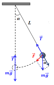
The specifics of this example is that the movement of a pendulum is constrained by a rigid rod, which necessitates introduction of constraints into a system of equations based on the Newton's Second law.
In the lecture Pendulum of this chapter we approached the task of finding the formula of this pendulum's movement using an angle of deviation of its rod from a vertical. We started analyzing the problem using Cartesian coordinates, but gave up noting the complexity of the problem.
This was not really the application of Newton's Second law. Actually, we used the non-Cartesian parameter (angle) to solve the problem, and we expressed the movement in terms of this angle, not the Cartesian coordinates of the pendulum's bob.
Let's try to move with Cartesian coordinates a little further to make sure that this is not a good way to approach this problem.
Here is how this task is supposed to be approached using the classical Newtonian approach.
Let x(t) and y(t) be time-dependent coordinates of a point-mass bob at the end of a rod moving along a circular trajectory. Assume, positive direction of the X-axis on a picture above goes to the right and positive direction of the Y-axis goes down.
Then an angle α of a deviation of a rod from a vertical is defined by
cos(α(t)) = y(t)/L
sin(α(t)) = x(t)/L
Two forces act on a bob of a pendulum:
(a) constant weight W directed vertically down along Y-axis, its projections on coordinate axes are:
Wx = 0
Wy = m·g
(b) tension of a rod T(t) that holds the bob on its end, its unknown magnitude is T(t) and its projections on coordinate axes are:
Tx(t) = −T(t)·sin(α) = −T·(x/L)
Ty(t) = −T(t)·cos(α) = −T·(y/L)
These parameters allow to construct differential equations of motion based on Newton's Second law
m·x"(t) = −T(t)·(x/L)
m·y"(t) = m·g − T(t)·(y/L)
In addition, we have to satisfy the constraint
x²(t) + y²(t) = L²
We have three equations with three unknowns x(t), y(t) and T(t).
We will skip (t) for brevity.
First, let's eliminate T by invariant transformations of the above equations.
(a) transfer m·g in the second equation to the left
m·x" = −T·(x/L)
m·y" − m·g = −T·(y/L)
(b) multiply the first equation by x, the second - by y and add them together
m·x·x" + m·y·y" − m·y·g =
= −T·(x²+y²)/L
(c) note that x²(t)+y²(t)=L², which allows to substitute it into the above equation and resolve it for T
m·x·x" + m·y·y" − m·y·g =
= −T·L
T = −(m/L)·(x·x" + y·y" − y·g)
(d) by differentiating an identity x²+y²=L² by time twice we get another identity:
2x·x' + 2y·y' = 0
x·x' + y·y' = 0
x'² + x·x" + y'² + y·y" = 0
x·x" + y·y" = −(x'² + y'²)
(e) use this in the expression for T above
T = (m/L)·(x'² + y'² + y·g)
(f) we can substitute T with its expression from (e) into original equations getting two equations with only two unknown functions x(t) and y(t) (mass m cancels out)
x"(t) = −(x/L²)·(x'²+y'²+y·g)
y"(t) = g−(y/L²)·(x'²+y'²+y·g)
The solution to the above system of differential equations is lengthy, it does not resolve into any elementary functions and the obtained integral as a solution is not pretty (it involves elliptical functions).
Let's forget about Cartesian coordinates and switch back to an angle as the main parameter.
It has two main advantages:
(a) there is only one parameter, not two like in Cartesian coordinates;
(b) there is no need to involve a constraint because it is implicitly built into an approach we took.
In the simplest form for the above example, two Cartesian parameters (x and y) minus one constraint
The above can be generalized to the following.
Consider a mechanical system moving in n-dimensional configuration space and described by n time-dependent coordinates:
s1,...,sn.
Assume, there are m constraints that affect the motion of this system
f(1)(s1,...,sn)=0,
...
f(m)(s1,...,sn)=0.
Then under certain conditions (see below) the movement of this system can be described by n−m generalized parameters, which means that the system has n−m degrees of freedom.
These conditions include:
(a) constraints must be holonomic (expressed as equations that contain functions of only coordinates and time, not the velocities or other non-positional parameters);
(b) constraints must be independent (not derived from one another) which for holonomic constraints would follow from the requirement of linear independency of their gradients.
It should be noted that each individual constraint, provided its gradient is nonzero, defines a surface (a smooth manifold of dimension n−1) in a configuration space.
A trajectory of a system constrained by m holonomic constraints with linearly independent gradients belongs to an intersection of all such surfaces (which is a smooth manifold of dimension n−m) defined by all m constraints.
The system's velocity at any point on its trajectory must be tangential to this intersection of surfaces and, therefore, perpendicular to each constraint's gradient.
With m linearly independent gradients that together span an m-dimensional space, the tangent space where all trajectories belong to span orthogonal to it (n−m)-dimensional manifold, and generalized coordinates are just coordinates in this constrained manifold.
The rigorous mathematical proof of the above statement and exact specification of conditions of its applicability are beyond the scope if this course.
However, some geometric interpretation might be helpful.
Imagine the n-dimensional Euclidean space Rn and a single constraint in it
f(s1,...,sn) = 0
For example, for a movement of a single point-mass we use n=3, our own three-dimensional space R3 with Cartesian coordinates x, y and z in it and a constraint - an equation of a sphere of radius r
x²+y²+z²=r².
The constraint means that the movement of our mechanical system expressed as coordinate functions of time si(t) (i∈[1,n]) is such that
f(s1(t),...,sn(t)) = 0
for any moment of time t.
In our example it means that a point-mass must be always on a surface of a sphere, which can be parameterized by only two parameters.
In general, under conditions described above, one constraint reduces the number of degrees of freedom of a mechanical system by one.

No comments:
Post a Comment