Unizor - Partial Derivatives - Definition

Notes to a video lecture on http://www.unizor.com

Partial Derivatives - Definition

A concept of partial derivative is applicable to functions of two and more arguments (we will consider it only for functions of two arguments) and is based on a concept of a derivative of a function of one argument that we are familiar with.

Graphically, a function of two arguments z=f(x,y) can be represented as a surface in a three-dimensional space.

If we fix one of the arguments, for instance, x=a, and consider our function for all values of the other argument y, while the fixed argument does not change its value, we will obtain a function of one argument f(a,y).

Similarly, if we fix another argument, y=b, and consider our function for all values of x, while the fixed argument y does not change its value, we will also obtain a function of one argument f(x,b).

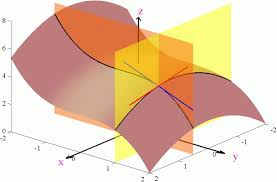
Graphically, we can see this function of one argument if we cut the graph of the original function z=f(x,y) by a plane x=a (or a plane y=b) and consider their intersection as a graph of this new function of one argument within plane x=a (or a plane y=b).

Here is an illustration of cutting a graph of a function of two arguments with a plane where x is fixed or by a plane where y is fixed:

For any real a we can analyze the behavior of function of one argument f(a,y), using familiar apparatus of differential calculus. For example, we can find points of maximum, minimum or inflection, intervals of increasing or decreasing etc.

In particular, we can find a derivative of this function, which is called a partial derivative of function z=f(x,y) by y.
In our description it depends on constant a (or a might get canceled in the process of differentiation as a constant, but this is irrelevant).

For example, function f(x,y)=x²+y² for x=a looks like a²+y² (where a is constant) and it has a partial derivative by y equal to 2y.
Function f(x,y)=x²·y³ for x=a looks like a²·y³ (where a is constant) and it has a partial derivative by y equal to a²·3y²=3a²y².

Traditionally, when talking about partial derivatives, we don't emphasize that one of the variables takes some special value (in our example, x=a), just that it is fixed, while we take a derivative by another variables. So, we don't substitute x=a before taking a partial derivative, we just assume that x (or y) is constant and then take a derivative by a variable that is not fixed.

So, for f(x,y)=x²+y² the partial derivative by y (assuming x is constant) is 2y, partial derivative by x (assuming y is constant) is 2x.
For f(x,y)=x²·y³ the partial derivative by y (assuming x is constant) is 3x²·y² and partial derivative by x (assuming y is constant) is 2x·y³.

We will also use symbols ∂/∂x and ∂/∂y to signify partial derivatives by x (keeping y fixed) and by y (keeping x fixed), correspondingly.
So, for function z=x²+y² we can write
∂z/∂x = 2x (y is considered constant)
∂z/∂y = 2y (x is considered constant)
For function z=x²·y³; we can write
∂z/∂x = 2x·y³ (y is considered constant)
∂z/∂y = 3x²·y² (x is considered constant)

Two important notes about this process of partial differentiation.

Note 1

After taking a partial derivative by any argument we obtain a function that can be partially differentiated again by any argument.
Thus, we can talk about partially differentiating twice by x or twice by y, or once by x and then by y, or once by y and then by x (order is important).

Using the symbolics suggested above and self explanatorily expanding it to derivatives of higher order, we can write:

∂²/∂x²(x²·y³) =
= ∂/∂x(∂/∂x (x²·y³)) =
= ∂/∂x (2x·y³) = 2y³

∂²/∂y²(x²·y³) =
= ∂/∂y(∂/∂y (x²·y³)) =
= ∂/∂y (3x²·y²) = 6x²·y

∂²/∂x∂y(x²·y³) =
= ∂/∂x(∂/∂y (x²·y³)) =
= ∂/∂x (3x²·y²) = 6x·y²

∂²/∂y∂x(x²·y³) =
= ∂/∂y(∂/∂x (x²·y³)) =
= ∂/∂y (2x·y³) = 6x·y²

The fact that two mixed partial derivatives (first by x then by y or first by y then by x) are the same in the above example is not a coincidence. There is a theorem that states that for a broad range of functions they are supposed to be the same. This will be addressed later.

Note 2

We can expand this definition of partial derivative to functions of any number of arguments. In all these cases we just have to assume that, partially differentiating by one argument, we assume all the others are constant.
For examples,
∂/∂x(x²+x·y) = 2x+y

Unizor - Definite Integrals - Improper Integrals Examples 2

Notes to a video lecture on http://www.unizor.com

Improper Definite Integrals

Example 2.1

∫₀¹2x/(1−x²) dx =
= lim_b→1 ∫₀^b2x/(1−x²) dx =
= lim_b→1 ∫₀^b1/(1−x²) d(x²)
Substitute t=x², including the limits of integration for t, which, considering x∈[0,b], would be t∈[0,b²].
The resulting integral would be
lim_b→1 ∫₀^b²1/(1−t) dt

Indefinite integral of function f(t)=1/(1−t) is F(t)=−ln(1−t).
Indeed, let's take a derivative of F(t)=−ln(1−t):
D_x F(t) = −(−1/(1−t)) = 1/(1−t)

Using Newton-Leibniz formula,
∫₀^b²1/(1−t) dx =
= F(b²) − F(0) =
= − ln(1−b²) + ln(1−0)
As b→1, ln(1−b²) is decreasing to negative infinity. So, this expression is increasing to positive infinity and we conclude that the original integral diverges.

Answer: This integral diverges, it has no real value.

__________

Example 2.2

∫₁^∞sin(1/x)/x² dx =
= lim_b→∞ ∫₁^bsin(1/x)/x² dx =
=lim_b→∞ −∫₁^bsin(1/x)d(1/x)=
= lim_b→∞ −∫₁^1/bsin(t)dt =
= lim_b→∞ ∫₁^1/b d(cos(t)) =
= lim_b→∞ [cos(1/b) − cos(1)]
As b→∞, this expression converges to 1 − cos(1)

Answer: 1 − cos(1)

__________


Example 2.3

Analyze the convergence of the following integral, depending on the value of parameter a.
∫₁^∞x^a dx

The indefinite integral of the function f(x)=x^a for any a≠−1 is F(x)=x^a+1/(a+1)
The case of a=−1 should be considered separately (see below).
Convergence of our integral for all cases when a≠−1 depends on convergence of the following limit:
lim_b→∞[F(b)−F(1)] =
= [1/(a+1)]·lim_b→∞[b^a+1−1]
Since infinitely increasing variable b in any positive power produces infinitely increasing variable, values of a that are greater than −1 should be excluded.
Infinitely increasing variable b, raised to a negative power will converge to zero.
Therefore, for all values of a that are less then −1 the limit will be −1/(a+1).
Consider now a case of a=−1.
Indefinite integral of function f(x)=x⁻¹=1/x is F(x)=ln(x)
Since this function is infinitely growing as x→∞, the original integral does not converge to any real number.

Answer:
This improper integral converges only for those values of parameter a that are less than −1, in which case the integral equals to
∫₁^∞x^a dx = −1/(a+1)
For example, for a=−2:
∫₁^∞x⁻² dx = ∫₁^∞1/x² dx = 1

__________


Example 2.4

Analyze the convergence of the following integral, depending on the value of parameter a.
∫₀¹x^a dx

First of all, for all positive values of parameter a this is a proper integral and its value is
∫₀¹x^a dx = 1/(a+1)
For a=0 our function f(x)=x^a is constant and equals to 1 everywhere except on the left margin x=0, where it is undefined.
So, we really have to calculate
lim_b→0∫_b¹x⁰ dx =
lim_b→0(1−b) = 1
(in which case the answer 1/(a+1) still valid).

Assume now that parameter a is negative. Obviously, in this case the function x^a grows to infinity as x→0, which makes our integral improper.
The indefinite integral of the function f(x)=x^a for any a≠−1 is F(x)=x^a+1/(a+1)
The case of a=−1 should be considered separately (see below).
Convergence of our integral for all cases when a≠−1 depends on convergence of the following limit:
lim_b→0[F(1)−F(b)] =
= [1/(a+1)]·lim_b→0[1−b^a+1]
Since infinitesimal variable b in any negative power produces infinitely growing variable, values of a that are less than −1 should be excluded.
Infinitesimal variable b, raised to a positive power will converge to zero.
Therefore, for all values of a that are greater then −1 the limit will be 1/(a+1).
Consider now a case of a=−1.
Indefinite integral of function f(x)=x⁻¹=1/x is F(x)=ln(x)
Since this function is infinitely decreasing to negative infinity as x→0, the original integral does not converge to any real number.

Answer:
This improper integral converges only for those values of parameter a that are greater than −1, in which case the integral equals to
∫₀¹x^a dx = 1/(a+1)
For example, for a=−1/2:
∫₀¹x^−1/2 dx = ∫₀¹1/√x dx = 2

Unizor - Definite Integrals - Improper Integrals Examples 1

Notes to a video lecture on http://www.unizor.com

Improper Definite Integrals

Example 1.1

∫₀¹1/√x dx =
= lim_a→0 ∫_a¹1/√x dx
Indefinite integral of f(x)=1/√x is F(x)=2√x.
Indeed, let's take a derivative of F(x)=2√x:
D_x F(x) = 2·(1/2)·x^(1/2)−1 =
= x^−1/2 = 1/√x

Using Newton-Leibniz formula,
∫_a¹1/√x dx = F(1) − F(a) =
= 2√1 − 2√a
As a→0, this expression converges to 2

Answer: 2

__________

Example 1.2

∫₀^∞e^−x dx =
= lim_b→∞ ∫₀^be^−x dx
Indefinite integral of f(x)=e^−x is F(x)=−e^−x.
Evaluating integral:
∫₀^be^−x dx = F(b) − F(0) =
= (−e^−b) − (−e⁻⁰) = 1 −e^−b
As b→∞, this expression converges to 1

Answer: 1

__________

Example 1.3

∫₀^∞1/(1+x²) dx =
= lim_b→∞ ∫₀^b1/(1+x²) dx
Indefinite integral of f(x)=1/(1+x²) is F(x)=arctan(x).
Evaluating integral:
∫₀^b1/(1+x²) dx = F(b) − F(0) =
= arctan(b) − arctan(0) =
= arctan(b)
As b→∞, this expression converges to π/2

Answer: π/2

__________

Example 1.4

∫₁^∞(1/x²)·e^1/x dx =
= lim_b→∞ ∫₁^b(1/x²)·e^1/x dx
Indefinite integral of
f(x)=(1/x²)·e^1/x can be found by noticing that −1/x² is a derivative of 1/x and, therefore, a derivative of e^1/x is e^1/x·(−1/x²).
Therefore, indefinite integral of f(x)=(1/x²)·e^1/x is F(x)=−e^1/x.
Evaluating integral:
∫₁^b(1/x²)·e^1/x dx = F(b)−F(1) =
= (−e^1/b) − (−e^1/1) = e − e^1/b
As b→∞, this expression converges to e −1

Answer: e −1

Unizor - Definite Integrals - Improper Integrals

Notes to a video lecture on http://www.unizor.com

Improper Definite Integrals

Recall the definition of the definite integral:
∫_a^bf(x) dx =
= lim Σ_i∈[1,N] f(x_i)·Δx_i
where Δx_i=x_i−x_i−1 represents partitioning of segment [a,b] into N parts, and it is assumed that the widest interval Δx_i is shrinking to zero by length as N→∞.

Before we only defined and calculated these integrals for cases where the segment of definition [a,b] was finite and the integrated function f(x) was, at least, continuous on this segment and, as a consequence, was finite as well.

Consider now cases of integration over unbounded (infinite) domains and/or functions that go to infinity around some point(s) within their domains. Let's start with a statement that we never defined these types of integrals. Riemann sums are not applicable in these cases.

For example, you want to determine an area under the curve y=1/x² from left boundary x=1 to positive infinity.
This function diminishes to zero as x→∞, so, intuitively, the area under this infinite curve might or might not be finite, depending on how fast the function value goes to zero as its argument goes to infinity.

Our first order is to define definite integrals of this kind.

Definition for infinite intervals of integration

We will define an improper integral of each kind as a limit of the corresponding proper integral if and only if this limit exists.

1. ∫_a^∞f(x) dx =
= lim_b→∞ ∫_a^bf(x) dx
provided this limit exists.

2. ∫^b_−∞ f(x) dx =
= lim_a→−∞ ∫_a^bf(x) dx
provided this limit exists.

When both margins are infinite, we can define the integral as a sum of two integrals, each with only one margin being infinite, provided both exists in a sense of corresponding limits as defined above.
3. ∫^∞_−∞ f(x) dx =
= ∫⁰_−∞ f(x) dx + ∫^∞₀ f(x) dx

Definition for functions going to infinity

Assume, we are integrating a function that asymptotically goes to infinity around one point within or on the border of a segment of integration.
For example,
∫₀¹ln(x) dx
As we know, logarithm goes to negative infinity as we approach argument 0, which is a left boundary of integration segment.
To define this integral, we will cut off this point out of integration by stepping side-wise and take a limit of the result as the point of cut-off is getting closer and closer to a point where our function is not defined. If this special point is on the border of a segment of integration, we will have to take only one such limit. If it's in the middle, we will have to split the segment in two parts and integrate each one separately using this technique.

Assume, function f(x) is defined and continuous on interval (a,b] that is open on the left because f(x)→∞ as x→a.
Then we define
4. ∫_a^bf(x) dx =
= lim_d→0 ∫^b_a+d f(x) dx
For any d, however small, integral on the right exists. So, if there is its limit as d→0, that limit is the definition of the integral on the left.

Analogously, assume, function f(x) is defined and continuous on interval [a,b) that is open on the right because f(x)→∞ as x→b.
Then we define
5. ∫_a^bf(x) dx =
= lim_d→0 ∫_a^b−df(x) dx
For any d, however small, integral on the right exists. So, if there is its limit as d→0, that limit is the definition of the integral on the left.

Finally, assume, function f(x) is defined and continuous on intervals [a,b) and (b,c] - everywhere at segment [a,c] except point x=b because f(x)→∞ as x→b.
Then we define
6. ∫_a^cf(x) dx =
= ∫_a^bf(x) dx + ∫_b^cf(x) dx
provided both integrals on the right exist in a sense of limits defined above.

_______

Example 1

∫₁^∞1/x² dx =
= lim_b→∞ ∫₁^b1/x² dx
The indefinite integral (antiderivative) of f(x)=1/x² is function g(x)=−1/x. Therefore, the definite integral on the right in the above equality can be evaluated by Newton-Leibniz formula as
∫₁^b1/x² dx =
= (−1/b) − (−1/1) = 1 − 1/b
Now we can take a limit of this expression as b→∞:
lim_b→∞ (1 −1/b) = 1
Therefore, according to the definition of this improper integral,
∫₁^∞1/x² dx = 1
_______

Example 2

∫₀¹ln(x) dx =
= lim_d→0 ∫_d¹ln(x) dx
Indefinite integral (antiderivative) of f(x)=ln(x) is g(x)=x·ln(x)−x (refer to a lecture about indefinite integrals or just differentiate this expression to check that its derivative is indeed equal to ln(x)).
Using Newton-Leibniz formula, we can evaluate the integral on the right:
∫_d¹ln(x) dx =
= (1·ln(1)−1) − (d·ln(d)−d) =
= −1 − d·ln(d) + d
Going to a limit as d→0, we notice that
lim_d→0 d·ln(d) = 0 (see a note with the proof below) and, therefore, our integral, according to the definition, is
∫₀¹ln(x) dx = −1
NOTE: Proof of the limit:
lim_d→0 d·ln(d) =
= lim_d→0 ln(d)/(1/d)
Use L'Hopital's rule to replace the ratio of functions with ratio of their derivatives.
lim_d→0 ln(d)/(1/d) =
= lim_d→0 (1/d)/(−1/d²) =
= lim_d→0 (−d) = 0

Unizor - Definite Integrals - Examples on Newton-Leibniz Formula

Notes to a video lecture on http://www.unizor.com

Definite Integrals -
Examples of Integration Using
Newton-Leibniz Formula

In this lecture we will consider exactly the same examples we used to demonstrate how definite integral can be calculated using its definition as a limit of sums.

Example 1

Find "area under curve" for f(x) = 10x on segment [a=0, b=4].

Solution

The indefinite integral (antiderivative) of function f(x) = 10x is 5x² (we can omit addition of a constant).
This function should be evaluated at the end points of integration resulting in the following:
∫₀⁴10x dx =
= 5·4² − 5·0² = 80−0 = 80
This corresponds to the answer we have obtained previously using limit of Riemann sums.
The end.
________________

Example 2

Find "area under curve" for f(x) = −x²+1 on segment [a=−1, b=1].

Solution

The indefinite integral (antiderivative) of function f(x) = −x²+1 is −x³/3+x (we can omit addition of a constant).
This function should be evaluated at the end points of integration resulting in the following:
∫₋₁¹(−x²+1) dx =
= [−(1)³/3+(1)] − [−(−1)³/3+(−1)] =
= 2/3 − (−2/3) = 4/3
This corresponds to the answer we have obtained previously using limit of Riemann sums.
The end.
________________

Example 3

The driver slows its car down by pressing the brakes from initial speed 20 meters per second to complete stop in 10 seconds, reducing its speed by the same value each second (linear dependency of the speed on time).
Find the distance the car covered during this breaking process.

Solution

First of all, we have to find the formula that represents the speed as a function of time.
Since every second the car slows down by the same number of meters per second, and it took 10 seconds to reduce the speed from 20 to 0, the function describing the speed is V(t)=20−2t.
The indefinite integral (antiderivative) of function V(t)=20−2t is 20t−t² (we can omit addition of a constant).
This function should be evaluated at the end points of integration [0,10] resulting in the following:
∫₀¹⁰(20−2t) dx =
= [20·10−10²] − [10·0−0²] =
= 100 − 0 = 100
The distance cover by car during breaking is 100 meters.
The end.
________________

Example 4

The Hooke's Law tells that a force needed to expand a string from its neutral position linearly depends on the length we expand it: F=K·x, where F is the force, x - the length of expansion and K - coefficient that depends on the physical properties of a spring.
Given a spring with K=0.5 (in newtons per meter).
Determine work W required to expand this spring by 0.1 meter.

Solution

Physical concept of work is defined as a product of a force by a distance this force is applied if this force is constant. In our case the force is changing with distance. To overcome this, we will approach this problem similarly to calculating an area under curve, where curve represents the force.
Partition the distance (spring's expansion) into small intervals and assume that the force is constant on each interval. If the force is a function of distance F(x) then the amount of its work from distance x=0 to distance x=d can be represented as
∫₀^dF(x) dx

Applying this to our case, we have to calculate
∫₀^0.10.5·x dx
The indefinite integral of function 0.5·x is 0.25·x².
Therefore,
W = ∫₀^0.10.5·x dx =
= 0.25·0.1² − 0.25·0² = 0.0025
The work equals to 0.0025(joules)
The end.

Unizor - Definite Integrals - Newton-Leibniz Formula

Notes to a video lecture on http://www.unizor.com

Definite Integrals -
Newton-Leibniz Formula

Recall the definition of the definite integral:
∫_a^bf(x) dx =
= lim Σ_i∈[1,N] f(x_i)·Δx_i
where Δx_i=x_i−x_i−1 represents partitioning of segment [a,b] into N parts, and it is assumed that the widest interval Δx_i is shrinking to zero by length as N→∞.

First Fundamental Theorem
of Calculus

Consider a smooth function f(x) on segment [a,b] and any point t∈[a,b].
The following definite integral can be considered as a function of t:
F(t) = ∫_a^tf(x) dx
The First Fundamental Theorem of Calculus states that the derivative of function F(t) is function f(t):
F^I(t) = f(t)

Proof

Since, by definition,
F^I(t) =
= lim_Δt→0[F(t+Δt)−F(t)] /Δt
we have to prove that
lim_Δt→0 [∫_a^t+Δtf(x) dx −
− ∫_a^tf(x) dx] /Δt = f(t)

From the properties of definite integrals we know that
∫_a^tf(x) dx + ∫_t^t+Δtf(x) dx =
= ∫_a^t+Δtf(x) dx
from which follows that
∫_a^t+Δtf(x) dx − ∫_a^tf(x) dx =
= ∫_t^t+Δtf(x) dx

Therefore, we have to prove that
lim_Δt→0 ∫_t^t+Δtf(x) dx /Δt = f(t)

From properties of definite integrals we know that
m·Δt ≤ ∫_t^t+Δtf(x) dx ≤ M·Δt
where m is minimum of function f(x) on segment [t,t+Δt] and M - its maximum on this segment.

This allows us to state that the expression
lim_Δt→0 ∫_t^t+Δtf(x) dx /Δt
is bounded from below by m (minimum f(t) on segment [t,t+Δt]) and from above by M (maximum f(t) on segment [t,t+Δt]).

As Δt→0, our segment [t,t+Δt] shrinks to a point t. Since we assume sufficient "smoothness" of function f(t) (in this case we need just its continuity), both minimum and maximum of f(t) on segment [t,t+Δt] converge to the same value f(t).
That forces the limit above also to converge to f(t).

End of proof.

IMPORTANT:
Since the derivative of function F(t) above (definite integral of function f(x) on a segment from a to t) equals to f(t), function F(t) can serve as an indefinite integral (antiderivative) of f(t).
Since we proved the existence and uniqueness of a definite (Riemann) integral for any continuous function, the theorem above has proven that for any continuous function there exists indefinite integral (its antiderivative).

Newton-Leibniz Formula

Let's assume that we want to find a definite (Riemann) integral ∫_a^bf(x) dx of some continuous function f(x) on segment [a,b].
Assume further that we know one particular function G(t) which is the indefinite integral (antiderivative) of f(t) (we deliberately decided to use different argument symbol t instead of x as an argument of function G(t) to have x only as a variable of integration).
That is, G^I(t) = f(t).

Recall that there are many functions, derivative of which equal to f(t), but we know that all of them differ from each other only by an addition of a constant.

So, on one hand we have G(t) as one of the possible indefinite integrals (antiderivative) of f(t).
On the other hand, we have just proven that derivative of
F(t) = ∫_a^tf(x) dx
by t also equals to function f(t).
Therefore, we have two different functions, derivatives of both of which are the same function f(t):
G^I(t) = f(t) and
F^I(t) = [∫_a^tf(x) dx]^I = f(t)

Since two antiderivatives differ only by an addition of a constant, we conclude that
F(t) = ∫_a^tf(x) dx = G(t) + C
where C - some constant.

It's easy to find this constant. Since a definite integral on a null-segment [a,a] equals to zero, assign t=a in the above formula getting
∫_a^af(x) dx = G(a) + C = 0
from which we get
C = −G(a)

The final formula for our definite integral, therefore, is
F(t) = ∫_a^tf(x) dx = G(t) − G(a)
In particular, for t=b, we obtain the Newton-Leibniz formula:
∫_a^bf(x) dx = G(b) − G(a)
where G(t) - any function, derivative of which is f(t), in other words, an indefinite integral (antiderivative) of f(t).

CONCLUSION

To find a definite integral of some real function f(t) on segment t∈[a,b], it is sufficient to find any particular indefinite integral (antiderivative) G(t) of function f(t) and calculate the expression G(b)−G(a).
This establishes a connection between indefinite and definite integrals and justifies the usage of the same word integral for both.

Unizor - Definite Integrals - Other Examples

Notes to a video lecture on http://www.unizor.com

Definite Integrals -
Other Examples

Distance

Consider the following problem.
A car moves along a straight line with variable speed given by function v(t) that defines speed v at any moment of time t.
Our task is to find the distance covered by this car from time moment t=a to moment t=b.

If the speed is constant v(t)=V, the solution is easy:
S = V·(b−a)

For variable speed the problem is not that easy. Here is what can be suggested as an approximate solution.
Let's divide our time interval [a,b] into N equal short intervals [a=t₀,t₁], [t₁,t₂], [t₂,t₃]... [t_N−1,t_N=b] and assume that during each interval the speed is not significantly changing - a reasonable assumption if the time interval is small enough.
Then the distance covered during i-th time interval [t_i−1,t_i] is approximately equal to
ΔS_i = v(t_i)·(t_i−t_i−1)
Here we use v(t_i) (the value on the right margin) as a constant speed during i-th time interval. We could have taken any other value during this interval - on the left margin, minimum on this interval, maximum or any in-between.

Notice that the approach is absolutely equivalent to our approach of finding the area under curve in the previous lecture.

Our next step is to summarize all ΔS_i to get a total distance and go to a limit as the number of intervals we divide our total travel time increases to infinity.
So, the final formula is
S = lim Σ_i∈[1,N] v(t_i)·(t_i−t_i−1) =
= lim Σ_i∈[1,N] v(t_i)·Δt_i
where limit is assumed to be taken when N→∞ and maximum width among all intervals Δt_i diminishes to zero.

As with a problem of area under curve, we can prove that the limit is independent of which point within each interval is used to get the speed value. This limit is also independent on how we break the total time travel into shorter intervals as long as the length of the longest among intervals is shrinking to zero as we proceed with dividing the total travel time into more and more intervals.


Draining

Consider the following problem.
There is a tub filled with water. When we open the drain, the water starts flowing out of the tub. The speed of water flow depends on different factors - some constant (the size of a drain pipe) and some variable (the pressure at the drain opening).

Our task is to determine the volume of water that is drained from the tub during some known period of time from t=a to t=b, provided we know the speed of draining v(t) (in some units, like liters per second) at any moment of time t.

The complication here, obviously, is that the speed of water flow through a drain is variable because it depends on the water pressure at the drain opening, which changes as the water flows out of the tub.

Our approach to this problem is similar to the one above.
Let's divide our time interval [a,b] into N equal short intervals [a=t₀,t₁], [t₁,t₂], [t₂,t₃]... [t_N−1,t_N=b] and assume that during each interval the speed of water flow through a drain is not significantly changing - a reasonable assumption if the time interval is small enough.
Then the volume of water going through a drain during i-th time interval [t_i−1,t_i] is approximately equal to
ΔW_i = v(t_i)·(t_i−t_i−1)
Here we use v(t_i) (the value on the right margin) as a constant speed during i-th time interval. We could have taken any other value during this interval - on the left margin, minimum on this interval, maximum or any in-between.

Notice that the approach is absolutely equivalent to our approach of finding the area under curve in the previous lecture.

Our next step is to summarize all ΔW_i to get a total volume of drained water and go to a limit as the number of intervals we divide our total drainage time increases to infinity.
So, the final formula is
W = lim Σ_i∈[1,N] v(t_i)·(t_i−t_i−1) =
= lim Σ_i∈[1,N] v(t_i)·Δt_i
where limit is assumed to be taken when N→∞ and maximum width among all intervals Δt_i diminishes to zero.

As with a problem of area under curve, we can prove that this limit is independent of which point within each interval is used to get the speed value. This limit is also independent on how we break the total time of drainage into shorter intervals as long as the length of the longest among intervals is shrinking to zero as we proceed with dividing the total time into more and more intervals.


Volume of Solids of Revolution

Consider the following problem.
There is a solid obtained by a revolution of some curve on a plane around an axis which also lies on this plane.
Let's assume that the curve is defined as a graph of a smooth function y=f(x), where argument x varies from a to b, and the axis of rotation is the X-axis.

Our task is to determine the volume of this solid.

If our function is constant, that is f(x)=c, our solid is a cylinder of height H=b−a and radius equal to that constant c.
If function f(x) is linear (so, its graph is a straight line), our solid is a truncated cone of height H=b−a and radiuses of its two bases equal to R_a=f(a) and R_b=f(b).
In either of the above cases we know classic geometric formulas to calculate the volume of a solid.
The complexity of our problem, obviously, is that the shape of our solid is not one of those well known types.

Let's approach our problem analogously to determining the area under curve.
Let's divide our argument interval [a,b] into N equal short intervals [a=x₀,x₁], [x₁,x₂], [x₂,x₃]... [x_N−1,x_N=b] and assume that on each interval the value of function f(x) is not significantly changing - a reasonable assumption if the interval is small enough.

Replacing the function values on each interval [x_i−1,x_i] with a constant value at its right margin f(x_i) and rotating the obtained step-function around the X-axis, we obtain a different solid, but the one that approximates the original one to certain degree.
The approximation will be better if the number of intervals we divide segment [a,b] is increasing and the size of the largest interval diminishes to zero.

The result of rotation of a step-function on each interval will be a cylinder with height h_i=x_i−x_i−1 and radius f(x_i), its volume will be equal to
ΔV_i = π·f ²(x_i)·(x_i−x_i−1) =
= π·f ²(x_i)·Δx_i

Our next step is to summarize all ΔV_i to get a total volume of a solid and go to a limit as the number of intervals we divide our segment [a,b].
So, the final formula is
V = lim Σ_i∈[1,N] π·f ²(x_i)·Δx_i
where limit is assumed to be taken when N→∞ and maximum width among all intervals Δx_i diminishes to zero.

As with a problem of area under curve, we can prove that this limit is independent of which point within each interval is used to get the radius of a cylinder. This limit is also independent on how we break the total range of arguments into shorter intervals as long as the length of the longest among intervals is shrinking to zero as we proceed with dividing the total range into more and more intervals.


CONCLUSION

In all the cases we considered so far we came up with an expression
lim Σ_i∈[1,N] f(x_i)·Δx_i
where f(x) is some smooth function defined on a segment [a,b],
{x_i} is partitioning of segment [a,b] into N parts,
and we assume that N→∞ and the maximum width of intervals Δx_i=x_i−x_i−1 converges to zero.

We have also proven that this limit exists for any smooth function f(x), that it does not depend on how we partition our segment [a,b] (as long as the widest interval of division shrinks to zero length) and it does not depend on which point within each interval of division we use to determine the function value on this interval.