Thursday, December 22, 2016

Unizor - Derivatives - Limit of Sequence - Big O, Little o


Notes to a video lecture on http://www.unizor.com

Rate of Change: Big-O, Little-o

Consider two infinitely growing sequences
{n} and {n+1}.
Both are infinitely growing, the second one is always (for any order number n) greater than the first, so it is "bigger" in some sense.
But, if you compare the rate of their growth, it is, actually, the same. When one doubles in value, another almost doubles too and the difference gets proportionally smaller and smaller.
The difference between these sequences, as they grow, is always 1, but their values are getting larger and larger, so proportional difference is getting more and more negligible. For order number n=10 the difference of represents 10% of the value, for n=1000 the difference of represents only 0.1% of the value. This allows us to say that both sequence are growing at the same rate.

On the other hand, if you consider these infinitely growing sequences
{n} and {ln(n)},
you will soon see that proportional difference becomes larger and larger as growth much faster than ln(n). For order number n=10 the first sequence has value 10, while the second, approximately, has 2.3 - 77% difference. For n=1000 the first sequence has value 1000, while the second, approximately, has 6.9 - more than 99% difference. And this proportional difference is growing. This allows us to say that the first sequence growth proportionally faster than the second. The rate of growth of the first sequence is greater than of the second.

Similar situation is with infinitesimals.
Consider two infinitesimal sequences
{1/n} and {10/n}.
Both are infinitesimal, though the first one is always smaller. Proportional difference between them is always 9/n, which represents 900% of the value of the first sequence. It does not change and, therefore, we can say that these two infinitesimals are diminishing with the same speed.

On the other hand, if you consider these infinitesimals
{1/n} and {1/ln(n)},
you will see that proportional difference is increasing as 1/n converges to zero much faster than 1/ln(n). Indeed, with order number n=10 the first sequence equals 0.1, while the second, approximately, is 0.4343 - more than 300% difference. For n=100 the first sequence is 0.01, while the second, approximately, is 0.2174 - more than 2000% difference. For n=1000 the first sequence is 0.001, while the second is 0.1448 - more than 14000% difference.

To address the relative rate of growth for infinitely growing sequences or relative rate of diminishing for infinitesimal sequences, there is a special notation called Big-O and Little-o.
Big-O means similar rate of change, while Little-o means "smaller" in terms of rate of change (slower growth for infinitely growing and faster diminishing for infinitesimals).

It should be noted that many sources differentiate between relative rates of change bounded from above (where it's called Big-O), from below (where it's called Ω) and from both sides (where it's called Θ).
For our purposes we will use only Big-O and assume that it refers to a relative rate of change bounded from both upper and lower sides. The definition below clarifies the exact meaning of this.

Thus, considering infinitely growing sequences, we can say that
n+1 = O(n) - to indicate the same rate of change or the same order of growing,
ln(n) = o(n) - to indicate that ln(n) is "smaller" in a sense of the rate of growing of ln(n) to infinity is slower than the rate of growing of n.

For infinitesimal sequences we can say that
10/n = O(1/n) - to indicate that both infinitesimals are diminishing to zero with the same speed, their order of diminishing is the same,
1/n = o(1/ln(n)) - to indicate that 1/n is "smaller" in a sense of the rate of diminishing to zero of 1/n is faster than the rate of diminishing to zero of 1/ln(n).

Let's now define Big-O and Little-o more rigorously.

Consider two sequences
{Xn} and {Yn}.
Definition of Little-o is based on the behavior of their ratio {Xn/Yn} (assuming Yn≠0).
If this ratio is an infinitesimal sequence, we say that
Xn = o(Yn)
Symbolically, the rate of change of Xn is o(Yn) if
ε>0 ∃Nn ≥ N ⇒ |Xn/Yn| ≤ ε

Definition of Big-O for two positive infinitely growing or infinitesimal sequences {Xn} and {Yn} is also based on the ratio {Xn/Yn}.
If, after certain order number, it is bounded from both sides by positive numbers, we say that these two sequences are of the same rate of change (or of the same order).
Symbolically, the rate of change of Xn is O(Yn) if
∃ A > 0B > 0N:
n ≥ N ⇒ A ≤ Xn/Yn ≤ B

Examples

1. Infinitely Growing - O()
Xn = 2n²+n−1Yn = n²−1
Xn/Yn = (2n²+n−1)/(n²−1) =
[(2n²−2)+(n+1)]/(n²−1) =
2+[(n+1)/(n²−1)] =
2+[1/(n−1)]
The last expression is, obviously, limited between A=2 and B=3 for n ≥ 2.
Therefore, Xn is O(Yn).

2. Infinitesimals - O()
Xn = 1/nYn = n/(n²−1)
Xn/Yn = (n²−1)/n² =
1−1/n²
The last expression is, obviously, limited between A=0.5 and B=1 for n ≥ 2.
Therefore, Xn is O(Yn).

3. Infinitely growing - o()
Xn = ln(n)Yn = n
Xn/Yn = ln(n)/n = ln(n1/n)
Expression n1/n converges to 1.
Here is a proof (with a help of a trick).
Let Zn=n1/n−1.
Obviously, Zn ≥ 0.
Consider an expression
(1+Zn)n.
On one hand, it is equal to
(1+n1/n−1)n = n.
On the other hand, let's use Newton's binomial for it:
(1+Zn)n = Σi∈[0,n]CniZni
Replacing the left side with and leaving only one member of the sum on the right - the one with Zn2 - we come up with the following inequality:
n ≥ Cn2Zn2
Since Cn2 = n(n−1)/2,
n ≥ Zn2n(n−1)/2 or
Zn2 ≤ 2/(n−1),
which proves that Zn is an infinitesimal variable and, therefore, n1/n→1.
Therefore, ln(n1/n) is converging to 0.
Therefore, Xn is o(Yn).

4. Infinitesimals - o()
Xn = 1/2nYn = 1/n
Xn/Yn = n/2n;
The expression n/2n is converging to zero.
Here is a proof.
Use Newton's binomial for identity 2n = (1+1)n:
2n = Σi∈[0,n]Cni
Using only one member of the sum on the right, we come up with an inequality
2n ≥ n(n−1)/2
from which follows
n/2n ≤ 2/(n−1).
Therefore, n/2n is an infinitesimal.
Therefore, Xn is o(Yn).

.
Friday, December 16, 2016

Unizor - Derivatives - Normal to Parametric Curve


Notes to a video lecture on http://www.unizor.com

Normal to Parametric Curves

We continue dealing with a curve on the plane that is parametrically defined by two functions - its coordinates that depend on some parameter{x(t);y(t)}, where both functions x(t) and y(t) are given and differentiable.

Our task is to find an equation that describes the normal to this curve at some point {x0;y0} that corresponds to a parameter value t=t0, that is x0=x(t0) and y0=y(t0).

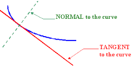
Geometrically speaking, a normal to a curve at some point is defined as a line perpendicular to a tangential line at that same point.
Here is how it looks.


Generally, a straight line that goes through point {x0;y0} has a point-slope equation
y−y0 = m·(x−x0)
So, all we have to determine in the equation for a normal that goes through point {x0;y0} is its slope m.

Since a normal to a curve at some point is, by definition, perpendicular to a tangential line at the same point, we can find the slope of a tangential line first and then turn the line by 90o.

From the previous lecture we know that the slope of a tangential line can be calculated as
m = Dt=t0[y(t)] /Dt=t0[x(t)]

If a tangential line forms angleθ with positive direction of the X-axis, and we have determined that tan θ = m (see formula form above), we can determine the angle ν formed by a normal that is perpendicular to a tangential line and positive direction of the X-axis as follows:
ν = θ−90o

Now we determine the slope of the normal using the following simple trigonometry:
n = tan(ν) = tan(θ−90o) =
= −tan(90o−θ) = −cot(θ) =
= −1/tan(θ) = −1/m =
= −
Dt=t0[x(t)] /Dt=t0[y(t)]
since cot(θ)=1/tan(θ) and assuming that derivatives, participating in these calculations, are not equal to zero at point t=t0.

The equation defining a normal will then look like this:
(y−y0) = −Dt=t0[x(t)](x−x0)/Dt=t0[y(t)]

Unizor - Derivatives - Parametric Curves


Notes to a video lecture on http://www.unizor.com

Differentiation
of Parametric Curves


Let's assume that we deal with some curve on the plane that is defined not as a graph of certain function that looks like y=f(x)(where x is abscissa and y - ordinate), but parametrically, where both coordinates are defined as functions of some parameter t.
An obvious example is a point moving on a plane, and its position {x;y} depends on a time parameter, so it can be described as {x(t);y(t)}, where both functions x(t) and y(t) are given and differentiable.
So, one independent parameter describes both coordinates through these two function.

Our task is to find an equation that describes the tangential line to this curve at some point{x0;y0} that corresponds to a parameter value t=t0, that is x0=x(t0) and y0=y(t0).

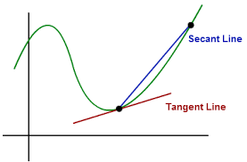
Geometrically speaking, a tangential line to a sufficiently smooth curve at some point is a limit of a secant line that intersects our curve at point where a tangential line should be and another point close to it, when that other point is getting closer and closer to the point of tangency.


Generally, a straight line that goes through point {x0;y0} has a point-slope equation
y−y0 = m·(x−x0)
So, all we have to determine in the equation for a tangential line that goes through point{x0;y0} is its slope m.

Since our tangential line is a limit of a secant, we can assume that the slope of a tangential line is the limit of a slope of a secant as the other point of secant's intersection with our curve is getting infinitesimally close to point {x0;y0}.

Consider a point of tangency{x0=x(t0);y0=y(t0)} and give an increment to parameter t from its value t0 to value t0+Δt.
The new point on a curve that corresponds to an incremented value of parameter t will be
{x1=x(t0+Δt);y1=y(t0+Δt)}

A secant that intersects our curve at points {x0;y0} and{x1;y1} has a slope equal to
m = (y1−y0)/(x1−x0)
which can be transformed into
m = Δy/Δx
where Δy=y(t0+Δt)−y(t0)
and Δx=x(t0+Δt)−x(t0)

Obviously, we want to express the limit of this expression for slope m as Δt→0 in terms of derivatives Dt[x(t)] and Dt[y(t)].
For this we can transform it into
m = y/Δt)/x/Δt)
from which follows that for Δt→0
m→m0=Dt=t0[y(t)] /Dt=t0[x(t)]
where derivatives are taken at point t=t0.

Example

A unit circle with a center at the origin of coordinates can be described parametrically with an angle θ from the positive direction of the X-axis to a radius to a point on a circle being a parameter. Let's use the radian measure of this angle.

Any point on a circle with coordinates {x;y} can be described through functions:
x=cos(θ),
y=sin(θ).

Let's choose a point that corresponds to a parameter value θ=π/4 and determine the equation of a tangential line at this point.
First of all, determine the coordinates of a point of tangency:
x=cos(π/4)=√2/2
y=sin(π/4)=√2/2
Now the slope should be equal to a ratio of derivatives of functions y(θ) and x(θ) at point with parameter θ=π/4:
Dθ=π/4[y(θ)]=Dθ=π/4[sin(θ)]=
cos(π/4) = √2/2
Dθ=π/4[x(θ)]=Dθ=π/4[cos(θ)]=
−sin(π/4) = −√2/2

The slope m of our tangential line is a ratio of the two values above:
m = (√2/2)/(−√2/2) = −1

So, the equation of our tangential line at point defined by parameter θ=π/4 in point-slope form is
y−√2/2 = −1·(x−√2/2)
or, in a standard form,
y = −x + √2

Tuesday, December 13, 2016

Unizor - Derivatives Example - arcsin(x)


Notes to a video lecture on http://www.unizor.com

Derivative Example -
Inverse Trigonometric Functions


f(x) = arcsin(x)

f I(x) = 1/1−x²


Proof

We will use the method ofimplicit differentiation to obtain the formula for a derivative of this function.

Let's start from a definition of function arcsin(x).

The domain of this function is[−1,1] and its values are in[−π/2,π/2].

Then, for any value of the argument x from its domain the function value y is defined as an angle in radians such that
(a) sin(y)=x
(b) −π/2 ≤ y ≤ π/2

The first statement can be expressed as
sin(arcsin(x))=x
Since these two functions,A(x)=sin(arcsin(x)) andB(x)=x, are equal within domain [−1,1], their derivatives are equal as well.

The derivative of the A(x) can be obtained using the chain rule for compounded functions.
AI(x)=d/dx[sin(arcsin(x))] =
cos(arcsin(x))·
d/dx[arcsin(x)]

The derivative of B(x) is trivial.
BI(x) = d/dx[x] = 1

From equality of these two derivatives we conclude
d/dx[arcsin(x)]=1/cos(arcsin(x))

Now let's analyze the expression cos(arcsin(x)).
We know that
sin(arcsin(x))=x and
arcsin(x)[−π/2,π/2].
Therefore,
cos(arcsin(x)) ≥ 0.
Hence,
cos(arcsin(x)) = √1−x²

The final formula for a derivative is
[arcsin(x)]I = 1/1−x²

A small detail remains whenx = ±1, which results in zero denominator. These are the points where our functionarcsin(x) is not differentiable.
Geometrically, it signifies that tangential lines at both ends,x=−1 and x=1, of the domain of function arcsin(x) are vertical, as can be seen from a graph of this function below:

Monday, December 12, 2016

Unizor - Derivatives - Implicit Differentiation


Notes to a video lecture on http://www.unizor.com

Implicit Differentiation

The method of implicit differentiation can be used to find a derivative of a function, implicitly defined by an equation that contains both argument and function value, for example
x² + y² = R²
where y is a function of x.

In some cases (like the one above) we can start from resolving the given equation for y as an explicit formula (like y = ±√R²−x²) and then take a derivative.
In other cases it might be impossible or impractical to resolve it for y, and these are the cases where implicit differentiation would be useful.

Consider the following problem, from which the method will be clear.

Problem 1

The function is given by the following implicit equation
x² + y² = sin(y)
that cannot be explicitly resolved for y.
Our purpose is to express the derivative dy/dx in terms of and y.

Solution

Assuming that y is some unknown function of x, we consider the defining equation as the equality between two functions: x² + y² and sin(y).
Since these two functions are equal, their derivatives must be equal as well:
[x² + y²]I = [sin(y)]I

Using the property of derivative of a sum and the chain rule for compound functions, this produces:
[]I + []I = [sin(y)]I
2·x + 2·y·yI = cos(y)·yI
This can be resolved for yI to get its expression in terms of and y:
yI = 2x/(cos(y)−2y)

Let's exemplify the method of implicit differentiation further.

Assume that we don't know how to differentiate a logarithmic function. Consider then the following problem.

Problem 2

Find the derivative of a function y = ln(x)

Solution

We know the definition of logarithmic function:
y = ln(x) means that
x = e y

On the left of the last equality is a function f(x)=x and on the right - a compound function g(x)=e y, where y=ln(x), derivative of which we want to calculate.
Let's differentiate both sides of the above expression using the chain rule for compound function ey:
Dx(x) = Dx(e y)
1 = e y·Dx(y)
Since e y = x by definition of logarithmic function y = ln(x), this results in
1 = x·Dx(y)
from which follows
Dx(y) = 1/x

Hence,
Dx(ln(x)) = 1/x
which is the same as we derived when calculated this derivative directly using the limits.

Problem 3

Find the derivative of a function y = xsin(x)

Solution

ln(y) = sin(x)·ln(x)
Dx(ln(y)) = Dx(sin(x)·ln(x))
(1/y)·Dx(y) = cos(x)·ln(x) + sin(x)·(1/x)
Dx(y) = y·[cos(x)·ln(x)+sin(x)·(1/x)]
Hence, derivative of xsin(x)equals to
xsin(x)·[cos(x)·ln(x)+sin(x)·(1/x)]

Thursday, December 8, 2016

Unizor - Derivatives - Function Limit - Extreme Value Theorem


Notes to a video lecture on http://www.unizor.com

Extreme Value Theorem

In this lecture we will consider real functions f(x) of real argument x defined on a closed segment.

We will prove the following theorem.

Extreme Value Theorem

continuous function defined on a segment (finite interval with endpoints) attains its extreme values.
In other words, there is at least one point within its domain where it reaches its maximum and there is at least one point where it reaches its minimum.

Proof

We will prove this theorem for a case of attaining the maximum value. The corresponding proof for minimum is completely analogous.

The proof is based on the boundedness theorem that states that any continuous function f(x) defined on segment [a,b] is bounded from above and below. It was proven in the previous lecture.

That means that a set of real values of our function {f(x)} is bounded from above. According to the axiom of completeness, there must be the least upper bound for this set of values.
Assume, M is this least upper bound for function f(x) on segment S1=[a,b]:
x[a,b] f(x) ≤ M

Consider now a set S2 of all points x in the domain of our function f(x), where the function value is greater than M−1/2.
This set cannot be empty because in this case M−1/2 would be an upper bound that is smaller than the least upper bound M.

Next, consider set S3 of all points x in the domain of our function f(x), where the function value is greater than M−1/3.
This set cannot be empty because in this case M−1/3 would be an upper bound that is smaller than the least upper bound M.
In addition, set S3 is a subset of set S2 since the restrictions on the values of function f(x) are more strict within this set.

Continue this process with set S4 of all points x in the domain of our function f(x), where the function value is greater than  M−1/4, set S5 of all points x in the domain of our function f(x), where the function value is greater than M−1/5 etc.
Generally, set Sn contains all points x in the domain of our function f(x), where the function value is greater than M−1/n.
Each of these sets cannot be empty because in this case M−1/n would be an upper bound that is smaller than the least upper bound M.
Every subsequent set Sn+1 is a subset of the previous set Ssince the restrictions on the values of function f(x) are more strict within this set:
S1S2S3⊃...⊃SnSn+1⊃...

Now we can pick a single point from each of these sets to obtain a bounded sequence of points {xn} within segment[a,b], which, according to Bolzano - Weierstrass theorem should have a convergent subsequence {yk} with the limit also lying within our closed segment [a,b]. Assume this limit is L.
This limit point L must be the point of maximum for function f(x), that is f(L)=M.

To prove this, consider the following:
Since yk→L as k→∞ and f(x) is continuous, f(yk)→f(L).
The distance between f(yk) and the least upper bound M is an infinitesimal as index increases to infinity because, if ykSk|f(yk)−M| ≤ 1/k.
Therefore, M must be the limit of f(yk), that is
M = limk→∞f(yk) = f(L)

As we have proven, the maximum M of function f(x) is attained at point L[a,b].

End of proof.

Wednesday, December 7, 2016

Unizor - Derivatives - Function Limit - Bounded Functions


Notes to a video lecture on http://www.unizor.com

Bounded Functions

In this lecture we will consider real functions f(x) of real argument x.
The domain of these functions will be a contiguous interval, finite or infinite, including or not including the endpoints.
A finite contiguous interval with endpoints included we will call segment.

We will prove the following theorem.

Boundedness Theorem

continuous function defined on a segment (finite interval with endpoints) is bounded from above and from below.

Proof

The proof is based on two main properties introduced in prior lectures:
(a) Bolzano - Weierstrass Theorem that states that from any bounded sequence we can extract a convergent subsequence.
(b) Continuity property.

We will only prove the boundedness from above, the one from below is completely analogous.

Let's assume the opposite, that our function f(x) is defined and continuous on segment [a,b], and is not bounded from above.
Then for any, however large, number N we will be able to find an argument xN[a,b] such that f(xN) ≥ N.

The sequence {xN} consists from points in segment [a,b]and, therefore, is bounded by the endpoints of this segment.
According to Bolzano - Weierstrass Theorem, we can extract from it a subsequence{yn} of points in this segment that converges to some pointY[a,b].
Since a set of values of our function is unbounded on sequence {xN}, it is also unbounded on subsequence {yn}and, therefore, there no limit off(yn) as n→∞.

But function f(x) is continuous on segment [a,b], which means that, if {yn}Y[a,b], then{f(yn)}f(Y). So, the limit off(yn) does exist.
Came to a contradiction. Hence,f(x) is bounded from above.

Unizor - Derivatives - Limit of Sequence - Bounded Sequence


Notes to a video lecture on http://www.unizor.com

Sequence Limit -
Bounded Sequence


A very important property of bounded sequences (those {xn}that can be "framed" in upper and lower bounds as A ≤ xn ≤ Bfor any n) is the following theorem.

Bolzano - Weierstrass Theorem

Any bounded sequence has a convergent subsequence.

Proof

Intuitively, an infinite sequence in a bounded space must have points of accumulation and, therefore, we can pick subsequence that converges to one of these points.
Rigorous proof requires some more precision.

Let's use the method of nested intervals.
Since A ≤ xn ≤ B for any n, we can state that infinite number of elements of our sequence are in the interval I1=[A,B].

Split our interval I1 in two equal parts at midpoint M1. Since original interval [A,B]has infinite number of members of our sequence, one of its halves or both must also contain an infinite number of them. Assume for definiteness that interval I2=[A,M1] is the one with infinite number of members of our sequence. Note that interval I2 is a subset of interval I1I1I2.

Split our interval I2 in two equal parts at midpoint M2. Since the "parent" interval[A,M1] has infinite number of members of our sequence, one of its halves or both must also contain an infinite number of them. Assume for definiteness that interval I3=[M2,M1] is the one with infinite number of members of our sequence. Note that interval I3 is a subset of interval I2I2I3.

This process of splitting intervals produces an infinite sequence of nested intervals:
I1I2I3⊃...⊃IkIk+1⊃...
Each subsequent interval is half the size of a previous interval and infinite number of members of our original sequence {xn} is located in each of them.

Let's choose any one point ykfrom each Ik. We will prove that this subsequence {yk} of the original sequence {xn}converges to some point inside interval [A,B].

Consider the left end of each of these intervals. Since intervals are nested, these left ends produce the monotonically increasing sequence of real numbers bounded from above by point B and, therefore, have a limit - point L1. This had been proven in "Algebra - Limits - Theoretical Problems" lecture of this course.
Similarly, consider the right end of each of these intervals. Since intervals are nested, these right ends produce the monotonically decreasing sequence of real numbers bounded from below by point A and, therefore, have a limit - point L2.
Since the length of our nested intervals converges to zero, it is obvious that points L1 and L2coincide. Let's call this one point L.

This point L is the also the limit of our subsequence {yk}because this subsequence is bounded from below by left ends of our nested intervals, bounded from above by their right ends, and these two bounding sequences of left and right ends converge to the same limit L. This had been proven in "Algebra - Limits - Theoretical Problems" lecture of this course.

End of proof.

Unizor - Combinatorics - Problem 2.9 - Vandermonde Identity


https://youtu.be/fxrut5Rbke0


Notes to a video lecture on http://www.unizor.com

Advanced Combinatorics - Problems 2.9.

Try to solve these problems yourself and check against the answers that immediately follow each problem.

Problem 1 - Vandermonde's identity

Prove the following identity for any natural numbers mn and r(where r ≤ m+n):
Cm+nr = Σi∈[0,r]Cmi·Cnr−i

Logic 1 (combinatorial):

Imagine, you have to pick a group of r people from a set of m men and n women.
One obvious answer is direct usage of the formula for a number of combinations of objects from m+n objects, regardless of men/women composition in the group. The answer in this case is Cm+nr, which is exactly an expression on the left of Vandermonde's identity.

On the other hand, we can differentiate groups by the number of men in them.
There are certain number of groups of r people with 0 men (and, correspondingly, r−0 women),
Then there are some groups with 1 man (and, correspondingly, r−1 women).
Some groups will have 2 men (and, correspondingly, r−2 women).
etc.
Some groups would have r−1 men (and, correspondingly, woman).
Finally, some groups will haver men (and, correspondingly, women).

The number of groups counted separately by the number of men and women should be equal to the number Cm+nr for the total number of groups we came up with counting them without regard to men/women composition.

Let's determine now how many groups can be chosen with exactly i men (and, correspondingly, r−i women) for each i from 0 to r and sum them up to get a total of groups of r people.
The number of groups of i men out of all m men is Cmi.
To each of these groups of i(out of m) men we can add any group of r−i (out of n) women (there are Cnr−i of them). So, the total number of groups composed of i men and r−i women equals to
Cmi·Cnr−i

Summarizing this by the number of men in a group from 0 to r, we should get the total number of groups Cm+nrof r people out of all m+n available that we calculated in the beginning:
Σi∈[0,r]Cmi·Cnr−i

The above is the right side of the Vandermonde's identity.
End of proof.

Logic 2 (algebraic):

We will use Newton's binomial formula
(a+b)k = Σi∈[0,k]Cki·ak−i·bi

Let's use it for the following three cases.
(a) a=1b=xk=m:
(1+x)m = Σi∈[0,m]Cmi·xi
(b) a=1b=xk=n:
(1+x)n = Σi∈[0,n]Cni·xi
(c) a=1b=xk=m+n:
(1+x)m+n = Σi∈[0,m+n]Cm+ni·xi

From obvious identity
(1+x)m+n = (1+x)m·(1+x)n
we derive the corresponding equality between
Σi∈[0,m+n]Cm+ni·xi
and the product of
Σi∈[0,m]Cmi·xi by
Σi∈[0,n]Cni·xi

The first one is a polynomial of(m+n)th power. The second is a product of a polynomial of mth power by a polynomial of nth power, which is, in theory, also a polynomial of (m+n)th power. So, since they are equal for any argument x, their coefficients atx at any particular power (from 0th to (m+n)th) should be the same.

The coefficients of the first polynomial are explicitly participating in the expression. Namely, for any r[0,m+n] a coefficient at xr equals to Cm+nr.

Since we have to compare this with a coefficient of a product of two polynomials of powers m and n with known coefficients, we have to come up with a coefficient of a product of two polynomials expressed in terms of coefficients of each one of them.
To obtain xr from a product of two polynomials, we can
take x0 from the first and xrfrom the second (with their corresponding coefficients Cm0and Cnr) AND
take x1 from the first and xr−1from the second (with their coefficients Cm1 and Cnr−1) AND
take x2 from the first and xr−2from the second (with their coefficients Cm2 and Cnr−2) AND etc.
take xr−1 from the first and x1from the second (with their coefficients Cmr−1 and Cn1) AND, finally,
take xr from the first and x0from the second (with their coefficients Cmr and Cn0)
and sum up all of these results getting xr with a coefficient
Σi∈[0,r]Cmi·Cnr−i
This coefficient at xr of the product of two polynomials(1+x)m and (1+x)n should be equal to a coefficient Cm+nr at xr of the polynomial 1+x)m+n.
That proves Vandermonde's identity.

Wednesday, November 30, 2016

Unizor - Derivatives - Intermediate Value Theorem


Notes to a video lecture on http://www.unizor.com

Intermediate Value Theorem

The intermediate value theorem is, probably, a result of attempts to find roots of equations, where direct formula for the roots is not available.
For example, consider you have to solve an equation
2^x + x³ = 0
There is no formula for solutions of this equation. Without contemporary computers it's not easy to solve it. Obviously, we can only hope to find the solutions approximately. So, it would be useful if we can determine an interval where the solution is located. The narrower interval - the better our understanding about the solution of this equation.

Notice that the left side of our equation is negative at x=−1:
2^(−1) + (−1)³ = 0.5−1 = −0.5
At the same time, it is positive for x=1:
2^1 + (1)³ = 2 + 1 = 3
Considering the left side of the equation is a continuous function and taking into account that it is negative at x=−1 and positive at x=1, it is intuitively obvious that somewhere in interval [−1,1] our function must cross the value of 0. Therefore, the solution to our equation must lie inside the interval [−1,1].

If we want to evaluate the solution more precisely, let's take a midpoint of this interval, point x=0, and check the sign of a function at this point:
2^0 + (0)³ = 1
It is positive. So, the solution to an equation must be within a narrower interval [−1,0] because a continuous function on the left side of our equation takes negative value −0.5 at the left end (x=−1) of this interval and positive value 1 at the right end (x=0) of this interval.

This process of dividing an interval in halves can be continued to get to a solution closer and closer. In practice, many algorithms of finding solutions to complicated equations are exactly as described here.

While we are interested in methodology of this approach, we are also interested in theoretical foundation of it.
Its base - Intermediate Value Theorem.

This theorem states:
If continuous function f(x) is defined on segment [a,b] and takes different values at the ends of this segment, f(a) ≠ f(b), then for any intermediate value C between f(a) and f(b) there is a point h between a and b, where function f(x) takes this intermediate value C.

Symbolically, for f(a) smaller than f(b), it looks like this:
∀C ∈ [f(a),f(b)] ⇒
⇒ ∃ h∈[a,b]: f(h) = C

Proof

The proof of this intuitively obvious theorem is not exactly straight forward and needs certain axiomatic foundation.
The main idea of this proof is based on the Completeness Axiom - the axiom that says that a set of real numbers is complete in the following sense.
Assume, there is a non-empty set of real numbers bounded from above.
Then Completeness Axiom states that there exists exactly one real least upper bound (called supremum) - a real number that is an upper bound and, at the same time, is less or equal to any other upper bound.

To understand why this axiom is called Completeness Axiom, here is a simple example illustrating that rational numbers are not a complete set in the above sense.
Indeed, consider a set of rational numbers that are bounded from above by condition X² ≤ 2. The supremum of this set is not a rational number (it is square root of 2). Therefore, rational numbers do not represent a complete set in the above sense.

The Intermediate Value Theorem deals with real numbers, and we assume that Completeness Axiom takes place.
Also assume for definiteness that f(a) is smaller than f(b).

Let's choose any number C between f(a) and f(b):
f(a) ≤ C ≤ f(b).
If C equals to f(a) or f(b), the theorem is trivial - we just take h=a or h=b, correspondingly. So, we can assume that C is strictly greater than f(a) and strictly less than f(b).

Consider now a set S of all real numbers {x} within segment [a,b] for which the value f(x) is not greater than C: f(x) ≤ C ⇒ x∈S.
This set S is not empty because, at least, point a belongs to it since f(a) ≤ C.

Set S is, obviously, bounded from above by real number b. Therefore, according to Completeness Axiom, set S has supremum - the least upper bound - number h.
Number h belongs to segment [a,b] because, if not, number b would be a smaller upper bound, which contradicts to the fact that h is the least upper bound.

Consider now value f(h). We will prove that f(h)=C and, therefore, h is the number, whose existence we have to prove.

If f(h) is smaller than C, continuous function f(x) will be smaller than C also in the immediate neighborhood of point h. Thus, using the definition of continuity, we can choose ε=[C−f(h)]/2 and find δ such that |x−h|≤δ ⇒ |f(x)−f(h)|≤ε.
Then we set x = h+δ and conclude:
f(h+δ) ≤ f(h)+ε.
Since
f(h)+ε = f(h)+[C−f(h)]/2 =
= C − [C−f(h)]/2 ≤ C,
it follows that
f(h+δ) ≤ C.
Therefore, h is no longer an upper bound of set S since h is smaller than h+δ and (h+δ)∈S.
Hence, f(h) cannot be smaller than C.

Somewhat similar logic can be applied in case f(h) is greater than C.
Continuous function f(x) will be greater than C also in the immediate neighborhood of point h. Thus, using the definition of continuity, we can choose ε=[f(h)−C]/2 and find δ such that |x−h|≤δ ⇒ |f(x)−f(h)|≤ε.
So, the value of function f(x) at all points within δ-neighborhood around point x=h is greater than C, thus containing no points of set S.
Therefore, all point of this C, to the left from point h and to the right of it, are upper bounds for set S, which is impossible since h is the least upper bound of set S, and no other upper bound points should be lying to the left of it.
Hence, f(h) cannot be greater than C.

The only possibility left is f(h)=C.
End of proof.

Monday, November 28, 2016

Unizor - Derivatives - Minimum or Maximum, or Inflection


Notes to a video lecture on http://www.unizor.com

Derivatives - MIN or MAX

We know that if a smooth function f(x), defined on interval (a,b) (finite or infinite) has a local maximum or minimum at some point x0, its derivative at this point equals to zero.

Consider the converse statement: if a derivative of a smooth function f(x), defined on interval (a,b), equals to zero at some point x0, it attains its local minimum or maximum at this point. Is it a correct statement?
The answer is NO.
Here is a simple example. Function f(x)=x³ is defined for all real arguments and is monotonically increasing, so it has no minimum and no maximum. Its derivative equals to f I(x) = 3x². It is non-negative, as the derivative of a monotonically increasing function should be, but, in particular, it is equal to zero at x=0.
So, a point where derivative equals to zero is not necessarily a point of minimum or maximum.

All points where a derivative equals to zero are called stationary points of a function. Some of them are points of local minimum, some - local maximum and others (not local minimums, nor maximums) are called inflection points.

Example of a local minimum is a function f(x) = x² at point x=0 with derivative f I(x) = 2x, which equals to zero at x=0.


Example of a local maximum is a function f(x) = −x² at point x=0 with derivative f I(x) = −2x, which equals to zero at x=0.


Example of a point of inflection is a function f(x) = x³ at point x=0 with derivative f I(x) = 3x², which equals to zero at x=0.


Our task now is to distinguish different kinds of stationary points of a smooth function, which ones are local minimums, which are maximums and which are inflection points.
To accomplish this, we need to analyze the behavior of both the first and the second derivatives of a function.

Examine the point of local minimum of a smooth function first. The fact that point x0 is a local minimum means that in the immediate neighborhood of this point the behavior of a function, as we increase the argument from some value on the left of x0 to some value on the right of x0, is to monotonically decrease its value, reaching minimum value at this point x0 and then to monotonically increase afterwards.
As we know, monotonically decreasing smooth functions have a non-positive derivative, while monotonically increasing - non-negative. Since in the immediate neighborhood of point x0 the only point where a derivative is equal to zero is only our point of local minimum x0, we conclude that a derivative to the left of a point of local minimum x0 is strictly negative and to the right of it - strictly positive. So, a derivative changes the sign from minus to plus going through a point of local minimum.
Therefore, our first tool to distinguish among different types of stationary points (those where a derivative equals to zero) is analyze the sign of a derivative to the immediate left and to the immediate right of a stationary point. If it changes from minus to plus, it's a point of local minimum.

In our first example above function f(x) = x² at stationary point x=0 has derivative f I(x) = 2x that changes the sign from minus to plus as we move from negative argument to positive over point x=0. That identifies stationary point x=0 as local minimum.

Analogously, it a derivative changes the sign from plus to minus in the immediate neighborhood of a stationary point, its a point of local maximum.

In our second example above function f(x) = −x² at stationary point x=0 has derivative f I(x) = −2x that changes the sign from plus to minus as we move from negative argument to positive over point x=0. That identifies stationary point x=0 as local maximum.

Finally, if a derivative does not change the sign, but, being negative on the left of stationary point, is increasing to zero at a stationary point and then goes negative again, it's an inflection point. Similarly, if a derivative does not change the sign, but, being positive on the left of stationary point, is decreasing to zero at a stationary point and then goes positive again, it's an inflection point as well.

In our third example above function f(x) = x³ at stationary point x=0 has derivative f I(x) = 3x² that does not change the sign as we move from negative argument to positive over point x=0. It's positive on both sides of a stationary point. That identifies stationary point x=0 as an inflection point.

Another approach to identify stationary points of a smooth function as local minimum, maximum or inflection points is to analyze the second derivative.

Assuming x0 is a stationary point of function f(x), that is f I(x0) = 0, let's check the function's second derivative at this point f II(x0). It can be positive, negative or zero.

If it's positive, it means that the first derivative (relative to which the second derivative of the original function is the first derivative) is monotonically increasing. Since the first derivative equals to zero at point x0, it must be negative to the left of this stationary point and positive to the right, that is it changes the sign from minus to plus and the stationary point is a local minimum.
In our first example of function f(x)=x² the second derivative is f II(x0) = 2 (constant), which at the stationary point x=0 equals to 2. It is positive, therefore we deal with local minimum.

If the second derivative at the stationary point is negative, it means that the first derivative (relative to which the second derivative of the original function is the first derivative) is monotonically decreasing. Since the first derivative equals to zero at point x0, it must be positive to the left of this stationary point and negative to the right, that is it changes the sign from plus to minus and the stationary point is a local maximum.
In our second example of function f(x)=−x² the second derivative is f II(x0) = −2 (constant), which at the stationary point x=0 equals to −2. It is negative, therefore we deal with local maximum.

Finally, if the second derivative is equal to zero at the stationary point, we cannot make any judgment looking on the value of the second derivative at the stationary point.
Consider function f(x)=x4. Its first derivative is f I(x0) = 4x³, it's equal to zero at x=0, so this is a stationary point. The second derivative is f II(x0) = 12x², which at the stationary point x=0 equals to zero. Since it's zero, we cannot identify this stationary point as local minimum, maximum or inflection, though visually it's a clear minimum. This illustrates that the method based on the value of a second derivative at the stationary point is not always working.

Unizor - Derivatives - Taylor Series


Notes to a video lecture on http://www.unizor.com

Derivatives - Taylor Series

Functions can be simple, like
f(x)=2x+3 or f(x)=x²−1
or more complex, like
f(x)=[x+ln(x)]1−sin(x)·etan(x+5)

Obviously, it is always easier to deal with simple functions. Unfortunately, sometimes real functions describing some processes are too complex to analyze at each value of its argument, and mathematicians recommend to approximate a complex function with another, much simpler to deal with.
And the favorite simplification is approximation of a function with a polynomial.

There is a very simple reason for this. Computer processors can perform calculations very fast, but their instruction set includes only four arithmetic operations. That makes it relatively easy to calculate the values of polynomials, but not such functions as sin(x) or ln(x) frequently occurred in real life problems.
Yet, we all know that computers do calculations involved with these functions. The way they do it is using the approximation of these and many other functions with polynomials.

Our task is to approximate any sufficiently smooth (in a sense of differentiability) function with a polynomial.
In particular, we will come up with a power series that converges to our function.
So, cutting this series on any member would produce an approximation with a polynomial, and the approximation would be better and better if we cut the series further and further from the beginning, increasing the number of elements participating in polynomial approximation.

First of all, we mentioned power series. Here we mean an infinite series, nth member of which is Cn·x n (where n=0, 1, 2...), which we can express as
P(x) = Σn≥0[Cn·x n].
Any finite series of this type is a polynomial itself and does not need any other simplification. So, we are talking about infinite series that has a value in a sense of the limit, when the number of members infinitely grows.

Obviously, not any power series of this type is convergent, but for sufficiently smooth functions defined on finite segment [a,b] there exists such a power series that converges to our function at each point of this segment, and we can achieve any quality of approximation by allowing sufficient number of members of a power series to participate in the approximation, that is cutting the tail of a series sufficiently far from the beginning.
Let's assign symbol PN(x) for a partial sum of the members of our series up to Nth power:
PN(x) = Σn∈[0,N][Cn·x n].
Using this symbolics,
P(x) = limN→∞PN(x)

Let's analyze the representation of a sufficiently smooth on segment [a,b] function f(x) with a power series P(x).
In particular, let's assume that we want to find coefficients Cn of such a power series that
(1) for some specific value of argument x = x0, called a center of expansion, any partial sum PN(x) has the same value as function f(x) regardless of how many members N participate in a sum, that is
∀N ≥ 0: f(x0)=PN(x0);
(2) this power series converges to our function for every argument x∈[a,b], that is f(x)=P(x).
The first requirement assures that, at least at one point x = x0 our approximation of a function with a partial power series will be exact, regardless of how long the series is.

Based on the first requirement for any partial sum of a power series at point x = x0, that is PN(x0), to be equal to the value of original function f(x0) at this point, it is convenient to represent our power sum as
P(x) = Σn≥0[Cn·(x−x0) n]
with C0=f(x0).
Now, no matter how close to the beginning we cut P(x) to PN(x), we see that
f(x0) = PN(x0) for all N ≥ 0.
The first requirement is, therefore, satisfied in this form of our power series.

Let's now concentrate on the second requirement for P(x) to converge to f(x) for any point x of a segment [a,b].
We will do it in two steps.
Step 1 would assume that P(x) does converge to f(x) at any point. Based on this assumption, we will determine all the coefficients Cn. In a way, these specific values of coefficients are a necessary condition for equality between P(x) and f(x).
On the step 2, knowing that coefficients Cn of a power series P(x) must have certain values derived in step 1, we will discuss the issue of convergence.

So, assume the following is true:
f(x) = Σn≥0[Cn·(x−x0) n].
As we have already determined, C0=f(x0).
Let's differentiate both sides of the equality above.
A member C0·(x−x0)0 will disappear during differentiation since it's a constant and any member of type K·(x−x0)k will become k·K·(x−x0)k−1.
So, the resulting equality will look like this:
f I(x) = Σn≥1[nCn(x−x0)n−1].
This is an equality that is supposed to be true for any argument x. Substituting x=x0, all members of the infinite series except the first one will be zero. The first one is equal to
1·C1·(x−x0)0 and, since the exponent is 0, we have the following equality:
f I(x0) = 1·C1
Now we know the value of the next coefficient in our infinite series:
C1=f I(x0) / 1

The next procedure repeats the previous one. Let's take another derivative.
A member 1·C1·(x−x0)0 will disappear during differentiation since it's a constant and any member of type K·(x−x0)k will become k·K·(x−x0)k−1.
So, the resulting equality will look like this:
f II(x) =
= Σn≥2[n(n−1)Cn(x−x0)n−2].
This is an equality that is supposed to be true for any argument x. Substituting x=x0, all members of the infinite series except the first one will be zero. The first one is equal to
2·1·C2·(x−x0)0 and, since the exponent is 0, we have the following equality:
f II(x0) = 1·2·C2
Now we know the value of the next coefficient in our infinite series:
C2=f II(x0) / (1·2)

It can easily be seen that the repetition of the same procedure leads to the following values of coefficients Cn of our series:
C3=f III(x0) / (1·2·3)
C4=f IV(x0) / (1·2·3·4)
and, in general,
Cn=f (n)(x0) / (n!)
where f (n)(x0) signifies nth derivative at point x0 (with 0th derivative being an original function) and n! is "n factorial" - a product of all integer numbers from 1 to n with 0! being equal to 1 by definition.

We came up with the following form of representation of a function f(x) as a power series:
f(x)=Σn≥0[f (n)(x0)·(x−x0)n/(n!)]
This representation is called Taylor series.
Sometimes, in case of x0=0, it is referred to as Maclaurin series.

This form satisfies the first requirement we set in the beginning: for a center of expansion x = x0 any partial sum of this series has the same value as function f(x) regardless of how many members N participate in a sum.

We can also say that, if there is a power series converging to our function for every argument x∈[a,b], it must have a form above with coefficients as derived.

Our next task is to examine conditions under which the power series above exists and converges.

Obvious first requirement is infinite differentiability of the function f(x) since the coefficients of our series contain derivatives to any level.

As for convergence, it depends on the values of derivatives at point x0. A reasonable assumption might be that derivative f (n)(x0) for any level (n) is bounded by some maximum value M:
|f (n)(x0)| ≤ M
Let's prove that in this case the series converges.

Assuming the above boundary for derivatives of any level at point x0, the problem of convergence is reduced to proving that the following series is converging for any c:
S(c) = Σn≥0 cn/n!

Theorem
A sequence cn/n!, where c is any positive constant and n is an infinitely increasing index number, is bounded by a geometric progression with a positive quotient smaller than 1, starting at some index m.

Proof
Choose an integer m greater than c and start analyzing the members of this sequence with index numbers n greater than index m.
The following inequalities are true then:
cn/n! ≤ cn−m·cm/[n·(n−1)·...
...·(m+1)·m!] ≤
≤ cn−m·cm/[mn−m·m!] =
= (c/m)n−m·Q
where constant Q equals to
Q = cm/m!
The last expression represents a geometric progression with the first member Q·c/m and quotient c/m. Since m was chosen as an integer greater than c, the quotient of this geometric progression is less than 1.
End of proof.

Now we see that the members of polynomial series we considered above are bounded by members of a geometric progression with positive quotient smaller than 1. For geometric progressions that is a sufficient condition for their sum to converge. Therefore, the polynomial series is convergent.
This convergence, as was mentioned above, is true under assumption that all derivatives of the original function f(x) at point x0 are bounded by some constant M.

This condition on derivatives can be weakened in different ways, which we will not mention here. Also open remains a question of precision of the approximation with partial sums of a polynomial series. There are different approaches to evaluation of the quality of this approximation, that we leave for self-study.

Unizor - Derivatives - One-Sided Function Limits


Notes to a video lecture on http://www.unizor.com

One-sided Function Limit

Definition 1
Real number L is the limit of function f(x) from the right (or is the right limit) as argument x approaches real number a if for any sequence {xn}, that approaches a while each element of this sequence is greater than a, the sequence {f(xn} converges to L.
Symbolically, it looks like this: limx→a+ f(x)=L
An equivalent definition using ε-δ formulation is as follows:
∀ε>0 ∃δ:
x∈(a,a+δ) ⇒ |f(x)−L| ≤ ε

Similar definition exists for the limit from the left.
Definition 2
Real number L is the limit of function f(x) from the left (or is the left limit) as argument x approaches real number a if for any sequence {xn}, that approaches a while each element of this sequence is less than a, the sequence {f(xn} converges to L.
Symbolically, it looks like this: limx→a− f(x)=L
An equivalent definition using ε-δ formulation is as follows:
∀ε>0 ∃δ:
x∈(a−δ,a) ⇒ |f(x)−L| ≤ ε

Theorem
If function f(x) converges to L as x→a, then this function converges to the same L as x→a+ or x→a−.

Proof
Both one-sided limits are supposed to be the same as a general limit. This follows from the fact that if f(xn)→L for any sequence of arguments {xn} approaching a, the same limit would be if arguments approach a only from the right or only from the left.

The converse statement is not, generally speaking, true.
For example, consider a function that is equal to 0 for all negative arguments and is equal to 1 for positive or zero arguments. This function has limit from the left 0 and limit from the right is 1.

However, if both one-sided limits exist and equal to each other, the general limit also exists and equal to these one-sided limits.

Theorem
Assume the following:
limx→a− f(x) = limx→a+ f(x) = L
Prove that
limx→a f(x) = L

Proof
Choose any positive constant ε.
Then we know that
∃δ1:x∈(a−δ1,a) ⇒ |f(x)−L| ≤ ε
and
∃δ2:x∈(a,a+δ2) ⇒ |f(x)−L| ≤ ε
Let δ=MIN(δ1,δ2).
Then both above conditions are met for this δ and we can state that
∃δ:x∈(a−δ,a+δ) ⇒ |f(x)−L| ≤ ε
which is the definition of a general limit at point x=a.

Monday, November 21, 2016

Unizor Derivatives - Constant Functions


Notes to a video lecture on http://www.unizor.com

Derivatives - Constant Function

The following statement is obvious.
If a smooth function f(x), defined on segment [a,b] (including endpoints), is constant, that is if
∀ x∈[a,b]: f(x)=f(a)=f(b),
then its derivative at any inner point of this interval equals to zero:
∀ x∈(a,b): f'(x) = 0

What is more interesting is the converse theorem.

Theorem 1

If a smooth function f(x), defined on segment [a,b] (including endpoints), has a derivative at any inner point equaled to zero, that is if
∀ x∈(a,b): f'(x) = 0,
then this function is constant on this segment, that is
∀ x∈[a,b]: f(x)=f(a)=f(b).

Proof

Let's choose any point x inside interval (a,b).
Now use Lagrange Theorem for our function f(x) on an segment [a, x] that starts at point a and ends at point x.
This theorem states that there exists a point x0∈(a, x) such that
f'(x0) = [f(x)−f(a)] / (x−a)
Since we know that the derivative of function f(x) on an interval (a,b) is zero at any point, we conclude that
0 = [f(x)−f(a)] / (x−a)
from which follows
f(x)=f(a).
Recall that point x was chosen as any point in interval (a,b). It means that f(x)=f(a) is true for any inner point of this interval.
Since function f(x) is smooth (which, in particular, implies continuity), the values at the end of this interval are also the same.
Hence, our function is constant on segment [a,b].

End of proof.

Theorem 2

If two smooth functions f(x) and g(x), defined on segment [a,b] (including endpoints), have equal derivatives, that is if
∀ x∈(a,b): f'(x) = g'(x)
then these functions are different only by a constant on this segment, that is
∃c:∀ x∈[a,b]: f(x)=g(x)+c.

Proof

Consider a new function
h(x)=f(x)−g(x).
Since derivatives of f(x) and g(x) are equal to each other, derivative of h(x) equals to zero as well:
h'(x) = f'(x)−g'(x)=0.
Now use the theorem above that states that if a smooth function h(x) has derivative equaled to zero at any inner point of a segment [a,b], then it is constant on this segment, that is
h(x) = c, where c=h(a)=h(b)
Therefore,
f(x)−g(x)=c for any x∈[a,b].

End of proof.

Important corollary
If we are given a derivative of some function and we have guessed an original function, from which this derivative was taken, we can say that any other function with the same derivative differs from the one we have guessed by a constant, and there are no other functions with this derivative.
For example, we can guess that, if derivative is f I(x)=x², then original function might be f(x)=x³/3. Now, based on the above theorem, we can state that an expression f(x)=x³/3+c describes all the functions that have derivative f I(x)=x², where c - any real number, and no other function with this derivative exists.

Friday, November 18, 2016

Unizor Derivatives - Cauchy Theorem


Notes to a video lecture on http://www.unizor.com

Derivatives -
Caushy Mean Value Theorem

Cauchy Mean Value Theorem

For two smooth functions f(x) and g(x), defined on segment [a,b] (including endpoints), there exist a point x0∈[a,b] such that the following is true:
f'(x0)/g'(x0) = [f(b)−f(a)]/[g(b)−g(a)]
(with obvious restrictions on denominators not equal to zero).

Proof

Proof of this theorem is based on Rolle's Theorem.
Consider a new function h(x) defined as:
h(x) = f(x) − g(x)·[f(b)−f(a)]/[g(b)−g(a)]

This function satisfies the conditions of Rolle's Theorem:
h(a) = f(a) −g(a)·[f(b)−f(a)]/[g(b)−g(a)] =
= [f(a)·g(b)−f(b)·(g(a)]/[g(b)−g(a)]
h(b) = f(b) − g(b)·[f(b)−f(a)]/[g(b)−g(a)] =
= [f(a)·g(b)−f(b)·(g(a)]/[g(b)−g(a)]

So, h(a) = h(b)

According to Rolle's Theorem, there exists point x0∈[a,b] such that
h'(x0) = 0

Let's find the derivative of function h(x) in terms of derivatives of the original functions f(x) and g(x):
h'(x) = f'(x) − g'(x)·[f(b)−f(a)]/[g(b)−g(a)]
Now the equality to 0 of the derivative of function h(x) at point x0 in terms of original functions f(x) and g(x) looks like this:
0 = f'(x0) − g'(x0)·[f(b)−f(a)]/[g(b)−g(a)]
from which follows
f'(x0)/g'(x0) = [f(b)−f(a)]/[g(b)−g(a)]

End of proof.

Unizor - Derivatives - Lagrange Theorem


Notes to a video lecture on http://www.unizor.com

Derivatives -
Lagrange Mean Value Theorem

Lagrange Mean Value Theorem

For a smooth function f(x), defined on segment [a,b] (including endpoints), there exist a point x0∈[a,b] such that
f'(x0) = [f(b)−f(a)]/(b−a)


Geometrically, this theorem states that there is a point x0 inside segment [a,b], where a tangential line is parallel to a chord connecting endpoints of function f(x) on this segment.

Proof

Proof of this theorem is based on Rolle's Theorem.
Consider a new function g(x) that is equal to a difference between f(x) and a chord connecting two endpoints of a function on segment [a,b]:
g(x) = f(x) −
−{(x−a)·[f(b)−f(a)]/(b−a)+f(a)}

This function satisfies the conditions of Rolle's Theorem:
g(a) = f(a) −
−{(a−a)·[f(b)−f(a)]/(b−a)+f(a)} = f(a) − f(a) = 0
g(b) = f(b) −
−{(b−a)·[f(b)−f(a)]/(b−a)+f(a)} = f(b) − [f(b)−f(a)+f(a)] = 0
So, g(a) = g(b) = 0

According to Rolle's Theorem, there exists point x0∈[a,b] such that
g'(x0) = 0

Let's find the derivative of function g(x) in terms of derivative of the original function f(x):
g'(x) = f I(x) − [f(b)−f(a)]/(b−a)
Now the equality to 0 of the derivative of function g(x) at point x0 in terms of original function f(x) looks like this:
f'(x0) − [f(b)−f(a)]/(b−a) = 0 from which follows
f'(x0) = [f(b)−f(a)]/(b−a)

End of proof.

Unizor - Derivatives - Rolle Theorem


Notes to a video lecture on http://www.unizor.com

Derivatives - Rolle Theorem

Rolle Theorem

If a smooth function f(x), defined on segment [a,b] (including endpoints), has equal values at both endpoints, that is f(a)=f(b), then there exists such point x0 ∈ [a,b] that its derivative at this point f I(x0) equals to zero:
f I(x0) = 0

Proof

Without pretending to be absolutely rigorous, the logical steps to prove this theorem might be as follows.

The function f(x) cannot be monotonically increasing because in this case its value at point x=b would be greater than that at point x=a.

Analogously, the function f(x) cannot be monotonically decreasing because in this case its value at point x=b would be less than that at point x=a.

Therefore, the function either is constant, in which case it's derivative at any internal point in the interval (a,b) equals to zero, or the function changes increasing to decreasing or decreasing to increasing behavior somewhere inside this interval.

Any point of change from increasing to decreasing is a local maximum, any point of change from decreasing to increasing is a local minimum. In both cases, according Fermat's Theorem, a derivative must be equal to zero at a point of change.

End of proof.

Unizor - Derivatives - Fermat Theorem


Notes to a video lecture on http://www.unizor.com

Derivatives - Fermat Theorem
(internal local extremums)

First of all, let's talk about terminology.

Internal local extremum is a term used to characterize the behavior of a function defined on some, maybe infinite, interval (a,b) without endpoints (to enable approach to any point of this interval from both sides without restrictions). That's why we use the word internal.

Next word that requires some clarification is local. This word is used to demonstrate that certain characteristics of a function can be observed at some point where it is defined and in the immediate neighborhood of this point. Thus, local maximum (minimum) is a point, where the value of a function is greater (less) than in any other point in some neighborhood of this point, even a very small one.

Finally, extremum is a word that means maximum or minimum. A point where local extremum is attained is called stationary point of a function.

Another important note is that we will consider only differentiable functions, those that have derivatives at each point. Moreover, we assume that these derivatives are continuous functions and, in some cases, differentiable themselves to obtain derivatives of the higher order.
Most functions considered in this course are of this type - polynomial, exponential, logarithmic, trigonometric functions and their combinations.

So, we will talk about local maximum or minimum of sufficiently smooth (in terms of differentiability) functions. This property of smoothness will be assumed by default, even if not explicitly specified.

Fermat Theorem

If a smooth function f(x), defined on interval (a,b), has local extremum at point x0, then its derivative at this point f I(x0) equals to zero:
f I(x0) = 0

Geometrically, since a derivative is related to a tangent of a tangential line to a function, its equality to zero means the horizontal tangential line at a point of local maximum or minimum. The following picture illustrates this.


Proof

Let's consider local maximum first.
Intuitively, local maximum of function f(x) at point x0 means that within some narrow neighborhood of x0, on the left of x0, function f(x) monotonically increases and on the right of it - monotonically decreases.
As was demonstrated before, monotonically increasing functions have non-negative derivative and monotonically decreasing functions have non-positive derivative. That necessitates that at x0 the derivative, a continuous function, as we mentioned above, must be equal to zero.
Here is an illustration:


A little more rigorously, we can assume that a derivative f I(x0) does not equal to zero. So, it's either positive or negative.
As was demonstrated earlier, if a derivative is positive at some point, the function at this point and in the immediate neighborhood of it must be monotonically increasing, thus it cannot have local maximum at this point (values on the left of this point are less then those on the right).
Similarly, if a derivative is negative at some point, the function at this point and in the immediate neighborhood of it must be monotonically decreasing, thus it cannot have local maximum at this point (values on the left of this point are greater then those on the right).
Therefore, a derivative at this point must be equal to zero.

The proof for local minimum is absolutely similar to this.
It would be a nice exercise to right down a proof of it without looking into the proof for maximum offered above.

End of proof.

Thursday, November 10, 2016

Unizor - Derivatives - Easy Problems


Notes to a video lecture on http://www.unizor.com

Derivatives - Easy Problems

We recommend to go through these easy problems before watching the lecture with their solutions.
We offer a simple proof of the first theorem as a sample.

Theorem 1

Assume, function f(x) is differentiable (that is, has a derivative) at some point x0.
Symbolically, the following limit exists and equals to some constant K:
limx→x0[f(x)−f(x0)]/(x−x0) = K
or, in a short form, setting
f(x)−f(x0) = Δf(x) and
x−x0 = Δx,
this looks as follows
limΔx→0[Δf(x)/Δx] = K
Prove that it is continuous at this point.

Proof

Given:
Δf(x)/Δx → K as Δx → 0.
Therefore,
β(x) = Δf(x)/Δx − K
is infinitesimal variable
as Δx → 0.
From this we derive that
Δf(x) = [K+β(x)]·Δx
is also an infinitesimal if Δx → 0.
This is a definition of continuity of function f(x) at point x0.

Theorem 2

Prove that monotonically increasing in some interval differentiable function has non-negative derivative in this interval.

Theorem 3

Prove that monotonically decreasing in some interval differentiable function has non-positive derivative in this interval.

Theorem 4

Prove that, if a derivative of a differentiable function is positive in some interval, the function is monotonically increasing in this interval.

Theorem 5

Prove that, if a derivative of a differentiable function is negative in some interval, the function is monotonically decreasing in this interval.