Unizor is a site where students can learn the high school math (and in the future some other subjects) in a thorough and rigorous way. It allows parents to enroll their children in educational programs and to control the learning process.
Find "area under curve" for f(x) = 10x on segment [a=0, b=4].
Solution
First, let's experiment with a couple of simple cases.
Case 1. N=2 Point of division in two equal parts is x1=2 So, a=x0=0, x1=2, x2=4=b Minimum on the first interval [0, 2] is 0 at x=0. Minimum on the second interval [2, 4] is 20 at x=2. Therefore, the sum of areas of all rectangles equals to S1 = 0·2 + 20·2 = 40.
Case 2. N=4 Two additional points of division in four equal parts are x1=1 and x3=3 So, a=x0=0, x1=1, x2=2, x3=3, x4=4=b Minimum on the first interval [0, 1] is 0 at x=0. Minimum on the second interval [1, 2] is 10 at x=1. Minimum on the third interval [2, 3] is 20 at x=2. Minimum on the fourth interval [3, 4] is 30 at x=3. Therefore, the sum of areas of all rectangles equals to S2 = 0·1 + 10·1 + + 20·1 + 30·1 = 60.
To proceed to a general case, assume we have divided our segment into N equal parts, and find the limit of the area of all rectangles as N→∞. In this case the width of each interval equals to Δxi = 4/N Right margin of i-th interval is xi = i·4/N The function value at this right margin is f(xi) = 10·i·4/N The area of the i-th rectangle, constructed on the i-th interval as a base and having height calculated above, equals to Si = 10·i·(4/N)·(4/N) = = (160/N²)·i
Our task is to sum these areas for i changing from 1 to N and find the limit of this sum as N→∞. Summation by i is simple, we did this before (see "Algebra - Sequence and Series" chapter of this course or prove the following by induction). Recall that Σ[1,K]i = K·(K+1)/2
Therefore, the result of summation of the areas of N rectangles is Σ[1,N]Si=(160/N²)·N·(N+1)/2= = 80·(1+(1/N))
As N→∞, this value converges to 80, which constitutes the "area under curve".
Incidentally, our "area under curve" can be calculated as the area of a right triangle with base 4 and height 10·4=40, which equals to S=(1/2)·4·40=80 - the same answer as we have received through rather complicated summation and taking the limit. That confirms the validity of our answer.
The end. ________________
Example 2
Find "area under curve" for f(x) = −x2+1 on segment [a=−1, b=1].
Solution
Again, let's consider two particular cases prior to generalize the problem. We will use the values of a function on the right margin of each interval.
Case 1. N=2 Point of division in two equal parts is x1=0 So, a=x0=−1, x1=0, x2=1=b The function value on the right margin of the first interval [−1, 0] is 1 at x=0. The function value on the right margin of the second interval [−1, 0] is 0 at x=1. Therefore, the sum of areas of all rectangles equals to S1 = 1·1 + 0·1 = 1.
Case 2. N=4 Two additional points of division in four equal parts are x1=−0.5 and x3=0.5 So, a=x0=−1, x1=−0.5, x2=0, x3=0.5, x4=1=b The function value on the right margin of the first interval [−1, −0.5] is 3/4 at x=−0.5. The function value on the right margin of the second interval [−0.5, 0] is 1 at x=0. The function value on the right margin of the third interval [0, 0.5] is 3/4 at x=0.5. The function value on the right margin of the fourth interval [0.5, 1] is 0 at x=1. Therefore, the sum of areas of all rectangles equals to S2 = (3/4)·0.5 + 1·0.5 + + (3/4)·0.5 + 0·0.5 = 5/4.
To proceed to a general case, assume we have divided our segment into N equal parts, and find the limit of the area of all rectangles as N→∞. In this case the width of each interval equals to Δxi = 2/N Right margin of i-th interval is xi = −1+i·2/N The function value at this right margin is f(xi) = 1−(−1+i·2/N)² = = (4/N)·i−(4/N²)·i² The area of the i-th rectangle, constructed on the i-th interval as a base and having height calculated above, equals to Si = Δxi·f(xi) = = (2/N)·[(4/N)·i−(4/N²)·i²] = = (8/N²)·i−(8/N³)·i²
Our task is to sum these areas for i changing from 1 to N and find the limit of this sum as N→∞. Recall that Σ[1,K]i = K·(K+1)/2 Σ[1,K]i² = K·(K+1)·(2K+1)/6
Therefore, the result of summation of the areas of N rectangles is Σ[1,N]Si = (8/N²)·(N·(N+1)/2 − − (8/N³)·N·(N+1)·(2N+1)/6
As N→∞, this value converges to 4−(16/6)=4/3, which constitutes the "area under curve".
Consider the following problem. Given a smooth function f(x) (we will always consider smooth functions in terms of continuity and sufficient differentiability), with non-negative values (that is, f(x) ≥ 0), defined on a closed segment [a, b] and represented by its graph on (X,Y) coordinate plane.
In the following we will use the word "area" in a sense of a two-dimensional part of a plane and as a quantitative measure of this part of plane. The context would clarify which one it is used in every case.
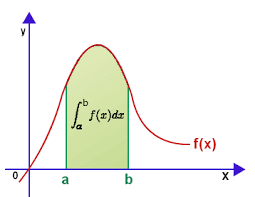
Our task is to find the "area under curve" - the measure of a part of coordinate plane bounded on the top by a graph of this function, on the bottom - the X-axis, on the left - by a line x = a and on the right - by a line x = b. This area looks like this gray shaded part of a plane (for now, do not pay attention to what's written inside this area):
There is no ready to use formula for such an area. We do know how the area of a rectangle is defined, it is a product of its two dimensions - length multiplied by width, but not of such a complicated figure as the one we consider now. We really have to define what the area of this figure is and then attempt to calculate it based on values of function f(x) on segment [a, b]. We did have a similar problem in Geometry with the area of a circle, and approached it as a sequence of approximations of a complex figure with simple ones. Let's do the same now.
We will use certain intuitive considerations to define the "area under curve" and will prove that this definition is mathematically valid.
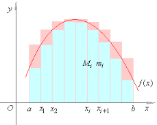
The process of approximation starts with dividing segment [a, b] into N intervals by points a=x0, x1, x2, x3...xN=b, and constructing rectangles, based on each interval [xi−1, xi], having the height equaled to a minimum value mi of function f(x) on this interval, similar to the following picture (consider only light blue rectangles)
All the light blue rectangles are completely below the curve (since their heights are minimums of the function values on each interval) and, therefore, the sum of their areas does not exceed the intuitively understood "area under curve".
Alternatively, we can consider a set of rectangles built on the same intervals but of the height equaled to a maximum value Mi of function f(x) on each interval (consider now pink extension of light blue rectangles). New taller rectangles are higher than the curve and, therefore, the sum of their areas is not less than the intuitively understood "area under curve".
Notice that the union of all blue rectangles resembles the figure we are trying to determine the area of. So, the sum of areas of all rectangles is close to the "area under curve", while always being less than "area under curve". This sum of areas of rectangles can be expressed by a formula sN = Σi∈[1,N]mi·(xi−xi−1) = Σi∈[1,N]mi·Δxi−1 where Δxi−1 = xi−xi−1, which is the width of each interval.
Adding pink extension, we note that the sum of these taller rectangles also approximates the "area under curve", while being larger than it. This sum of areas of rectangles can be expressed by a formula SN = Σi∈[1,N]Mi·(xi−xi−1) = Σi∈[1,N]Mi·Δxi−1 where Δxi−1 = xi−xi−1, which is the width of each interval.
Both approximations seem to be better if the number of intervals N we divide our segment [a, b] is large. And the larger is N - the better our approximation will be.
This can be confirmed by the following obvious statements. If we divide any existing interval in two parts, build two rectangles instead of one and calculate the sum of areas of these rectangles, sum sN, based on minimum values of function f(x), will increase and sum SN, based on maximum values of function f(x), will decrease.
Let's continue adding points of partitioning to infinity such that the largest interval's width converges to zero. During this process sum sN will monotonically increase or stay the same, but not decrease, while being bounded from above by any SN; and sum SNwill monotonically decrease or stay the same, but not increase, while being bounded from below by any sN. These properties of sequences sN and SN are sufficient to state that both have limits: limsN = s∞ limSN = S∞ where s∞ ≤ S∞, and the limit is understood in terms of making partitioning of segment [a, b] finer and finer with the largest interval shrinking in width to zero.
So, our next step in the process of approximation of the "area under curve" is to divide each of N intervals in two parts, getting twice as many intervals and build twice as many narrower rectangles. Blue rectangles lying below the curve will be inscribed "tighter" to the area under the graph of function f(x), so the approximation of the "area under curve" with sN will be better. Blue rectangles with pink extensions lying above the curve will encompass "tighter" the area under the graph of function f(x), so the approximation of the "area under curve" with SN will also be better.
As the number of intervals grows and the width of the largest interval becomes an infinitesimal variable, the difference between sN and SNbecomes smaller and smaller. If we can prove that this difference converges to zero, as long as the width of the largest interval converges to zero, it would be a sufficient foundation to call the limits s∞or S∞ (they are the same) the area under curve.
Proof
Recall that we are proving this theorem for sufficiently smooth functions. They and their derivatives are assumed to be continuous. In general, the theorem can be proven under weaker conditions (differentiability is not a necessary condition), but for the purposes of this course we are choosing the easier proof that is valid for smooth functions.
Consider the i-th interval [xi−1, xi]. Assume that function f(x) reaches its maximum Mi on this interval at point ξi∈[xi−1, xi] and it reaches its minimum mion this interval at point ηi∈[xi−1, xi].
According to Lagrange Mean Value Theorem, there is a point ζi∈[ξi, ηi]. such that f I(ζi)·(ξi−ηi) = Mi−mi from which we can derive the upper boundary for |Mi−mi|: |Mi−mi| ≤ max[a,b]{|f I(x)|} ·maxi{|xi−xi−1|}
Here max[a,b]{|f I(x)|} represents the maximum of the absolute value of the first derivative of f(x) on segment [a,b], which is some constant since f(x) is a smooth function, let's call it K. The second multiplier maxi{|xi−xi−1|} represents the maximum width of intervals in our partitioning of the original segment into N parts, let's call it WN.
So, we conclude that |Mi−mi| ≤ K·WN where WN (the widest interval) is assumed to be an infinitesimal variable as N→∞.
Now we can evaluate the difference SN−sN: SN−sN = Σi∈[1,N](Mi−mi)·(xi−xi−1) ≤ K·WN·Σi∈[1,N](xi−xi−1) = K·WN·(b−a)
The last expression contains an infinitesimal variable WN multiplied by two constants. Therefore, we have proven that the difference between upper SN and lower sN boundaries of "area under curve" is infinitesimal variable if the widest interval of partitioning of our segment [a,b] shrinks in width to zero.
From this follows that if, instead of choosing minimum value mi or maximum value Mi on each interval [xi−1,xi] as the height of a corresponding rectangle, we choose any value of a function f(x) on this interval, the limit will be the same since the corresponding sum of areas of these rectangles will always be between sN and SN.
We can conclude now that if we define the area under curve as a limit of sum of areas of rectangles based on intervals we divide the original segment into with the heights equal to values of our function in any point inside the corresponding intervals (left margin xi−1, right margin xi, maximum point ξi, minimum point ηi or any other), the limit will be the same as long as the widest interval's width converges to zero.
That proves the mathematical correctness of this definition. The area under curve, as defined, exists (since the limit of the sums of rectangles exist) and unique (since the limit does not depend on how we proceed partitioning the original segment and how we choose the points where the function value for the height of rectangle is chosen).
IMPORTANT: All these problems require certain guessing based on known rules of integration (substitution and "by parts") and recollection of derivatives of known functions. These problems are illustration of a notion of integration as a form of art more than a skill.
Problem 2.1:
∫dx / (cos(x)−sin(x))
One way to approach this problem was offered in a previous lecture and was based on the identity cos(x)−sin(x) = = (cos(x)·cos(π/4) − − sin(x)·sin(π/4)) / (√2/2) = = √2·cos(x+π/4) The result of the integration using this method was (√2/4)·[ln(1+sin(x+π/4)) − − ln(1−sin(x+π/4))] + C
Let's consider a different approach to "rationalize" this problem. Recall that all trigonometric functions can be expressed as rational functions of a tangent of a half-angle. In particular, sin(x) = = 2·tan(x/2) / (1+tan²(x/2)) cos(x) = = (1−tan²(x/2)) / (1+tan²(x/2)) From these identities we derive cos(x) − sin(x) = = (1−tan²(x/2)−2·tan(x/2)) / / (1+tan²(x/2)) and dx / (cos(x) − sin(x)) = = (1+tan²(x/2)) dx / / (1−tan²(x/2)−2·tan(x/2))
Derivative of tangent can also be expressed in terms of tangent: tanI(x) = 1+tan²(x) Therefore, d tan(x/2) = = (1/2)·(1+tan²(x/2)) dx and (1+tan²(x/2)) dx = = 2· d tan(x/2)
Therefore, our integral can be expressed in terms of an integral of some rational function of tangent as follows: ∫[2· d tan(x/2) / / (1−tan²(x/2)−2·tan(x/2))]
The numerator equals to: 1/cos²(x/2). The denominator equals to: [sin²(x/2)+2sin(x/2)·cos(x/2)− −cos²(x/2)]/cos²(x/2) The result of division of numerator by denominator, considering the minus sign in-front of the whole fraction, equals to: 1/[−sin²(x/2)− −2sin(x/2)·cos(x/2)+ +cos²(x/2)] = = 1/[cos(x)−sin(x)]
Since differentiation of our result proves that it's correct, it should differ from the result of the previous lecture for this integral by a constant.
Whoever suggests the trigonometric proof that the formula for a result from a previous lecture (√2/4)·[ln(1+sin(x+π/4)) − − ln(1−sin(x+π/4))] plus some constant equals to a new result (√2/2)·[ln(tan(x/2)+1+√2) − ln(tan(x/2)+1−√2)] will be mentioned in the notes for this lecture.
Problem 2.2:
∫dx / (cos(x)−sin(x))
Yes, still the same problem, but yet another approach to "rationalize" it.
Recall the wonderful Euler's formula that defines the exponential function of a complex argument: eix = cos(x) + i·sin(x) Using this formula, we can express both cos(x) and sin(x) as exponential functions of a complex argument as follows: e−ix = ei·(−x) = = cos(−x) + i·sin(−x) = = cos(x) − i·sin(x) Therefore, cos(x) = (1/2)·(eix+e−ix) sin(x) = (1/(2i))·(eix−e−ix) Since i² = −1, we can replace 1/i with −i and the last expression for sin(x) would look like this: sin(x) = −(i/2)·(eix−e−ix) = = (i/2)·(e−ix−eix)
We are planning to use this representation to reduce our integral to something familiar. The problem is, of course, that we never explained what is a derivative or an integral when dealing with functions that take real arguments but take complex values, as is the case with functions like eix. However, we will use the same techniques with these functions as we did with real functions. Strictly speaking, we have to prove that all these techniques are applicable (and they are!), but the procedures to prove all these properties are exactly the same as for real functions, So, we'll skip this and use all the available apparatus as if we have proven its applicability.
Notice that (1+i)/(1−i) = i because (1−i)·i = i−i² = 1+i Also, e2ix = (eix)² and e−ix = 1 / eix
That makes our denominator look like this: cos(x)−sin(x) = = (1−i)·[i·(eix)² +1] / (2·eix)
As we see, all depends now on eix. This prompts us to use substitution y=eix. We also have to express dx in terms of dy as follows: x = ln(y)/i = −i·ln(y) Therefore, dx = −i·dy / y Now our integral equals to ∫2·y·(−i·dy/y)/{(1−i)·[i·y² +1]} = = [−2i/(1−i)]·∫dy/[i·y² +1]
One more trivial substitution z=√i·y would result in the denominator within this integral to be equal to 1+z² familiar from differentiation of arctan(z). In this case dy=dz/√i and our integral equals to [−2√i/(1−i)]·∫dz/[z² +1]
The integral itself equals to arctan(z)+C. As for a multiplier, as was shown in the chapter "Complex Numbers" (and trivially checked directly), [(√2/2)·(i+1)]² = i So, we replace √i with (1+i)/√2 Also, as we saw above, (1+i)/(1−i) = i That simplifies the result of integration to −√2·i·arctan(z) + C
Reversing the substitutions, we get the following result of integration ∫dx / (cos(x)−sin(x)) = =−√2·i·arctan((i+1)·eix/√2)+C
Notice that, regardless of the presence of an imaginary i, this expression should be a real function. To prove it, we have to get deeper into functions of complex arguments, which is beyond the scope of this course.
IMPORTANT:
All these problems require certain guessing based on known rules of integration (substitution and "by parts") and recollection of derivatives of known functions.
These problems are illustration of a notion of integration as a form of art more than a skill.
Problem 1.1:
∫ sin(x)/cos³(x) dx
We know that (cos(x))I = −sin(x).
Therefore, we can combine sin(x) in the numerator and dx to obtain −dcos(x).
Our integral is transformed into −∫dcos(x)/cos³(x)
This substitution allows to integrate as if we have a power function ∫ xadx = xa+1/(a+1) where a=−3.
Since ∫dx/x³ = −1/(2x²)+C,
our integral equals to 1/(2cos²(x))+C
Checking the answer: (1/(2cos²(x)))I = (1/2)(1/cos²(x))I = (1/2)(−2/cos³(x))·(−sin(x)) = sin(x)/cos³(x).
The end.
Problem 1.2:
∫ ln(sin(x))·cot(x) dx
To find this integral, notice that cot(x) = cos(x)/sin(x)
Since (sin(x))I = cos(x),
we use sin(x) as an inner function: ln(sin(x))·cot(x) = ln(sin(x))·(sin(x))I/sin(x)
Next, notice that, since (ln(x))I = 1/x, (ln(sin(x)))I = (1/sin(x))·(sin(x))I
Therefore, ln(sin(x))·cot(x) = ln(sin(x))·(ln(sin(x)))I
Using the above substitution, we obtain the answer: ∫ ln(sin(x))·cot(x) dx = ∫ ln(sin(x))·dln(sin(x)) = ln²(sin(x))/2 + C
Checking by differentiating the answer: Dx (1/2)ln²(sin(x)) = ln(sin(x))·(1/sin(x))·cos(x) = ln(sin(x))·cot(x)
The end.
Problem 1.3:
∫ (ln(x)−3)/(x·√ln(x)) dx
To find this integral, break it in two integrals: ∫ ln(x)/(x·√ln(x)) dx −∫3/(x·√ln(x) dx) = ∫ √ln(x)dln(x) −∫3/√ln(x)dln(x) =
= (2/3)√ln³(x) − 6√ln(x) + C
Checking by differentiating the answer: Dx ((2/3)√ln³(x) − 6√ln(x)) = (2/3)·(3/2)·√ln(x)·(1/x) − 6·(1/2)·(1/√ln(x)·(1/x) = = (1/x)·(√ln(x) − 3/√ln(x)) = (ln(x)−3)/(x·√ln(x))
The end
Problem 1.4:
∫ x²·ex/2dx
Let's use the fact that exponential function does not change much with differentiation.
Transform our integral into ∫ 2x² dex/2
Now we can use integration by parts twice getting 2x²·ex/2 − 2∫ ex/2dx² = 2x²·ex/2 − 2∫ ex/2·2x dx = 2x²·ex/2 − 2∫ 2x·2 dex/2 = = 2x²·ex/2−8ex/2·x+8∫ ex/2dx = 2ex/2(x²−4x+8) + C
Checking by differentiating the answer: Dx (2ex/2(x²−4x+8)) = 2ex/2·(1/2)·(x²−4x+8) + 2ex/2·(2x−4) = = ex/2·(x²−4x+8+4x−8) = ex/2·x²
The end
Problem 1.5:
∫dx / √(−x²+4x+5)
Notice that arcsinI(x) = 1/√(1-x²)
The fact that a coefficient with x² is negative is very important. It prompts that we can try to transform our original function to be integrated into a form similar to a derivative of arcsin(x).
So, our task is to transform an expression under an integral into an expression that looks like the above derivative with linear transformation of variable x.
Basically, we have to express a quadratic polynomial under a square root as a full square expression. −x²+4x+5 = 9−(x−2)² = 9·(1−(x−2)²/9) = 9·(1−((x−2)/3)²)
Let's substitute y = (x−2)/3
Then x = 3y+2 and dx = 3dy
Then our integral looks like this: ∫ 3dy/√(9·(1−y²)) = ∫dy/√(1−y²) = arcsin(y) + C = arcsin((x−2)/3) + C
Checking by differentiating the answer: Dx arcsin((x−2)/3) = 1/(3√(1−((x−2)/3))²)) = 1/√(9−x²+4x-4) = 1/√(−x²+4x+5)
The end
Problem 1.6:
∫dx / (cos(x)−sin(x))
It's easy to deal with either cos(...) or sin(...).
To accomplish this, we can use the property cos(π/4)=sin(π/4)=√2/2
and transform the denominator into the following form: cos(x)−sin(x) = (cos(x)·cos(π/4) − sin(x)·sin(π/4)) / (√2/2) = √2·cos(x+π/4)
Substitute y = x+π/4.
Then dy = dx.
Our integral now looks like ∫dy / (√2·cos(y)) = (√2/2)∫dy / cos(y)
To find the above integral, we can multiply the nominator and denominator by sinI(y) = cos(y) and express everything in terms of sin(y): (√2/2)∫dsin(y) / (1−sin²(y))
New substitution z = sin(y) leads to the following integral: (√2/2)∫dz / (1−z²)
Now we can use an obvious identity 1 / (1−z²) = (1/2)·((1/(1−z) + 1/(1+z))
Our integral equals to a sum of two integrals: (√2/4)∫dz / (1−z) + (√2/4)∫dz / (1+z) = (√2/4)[−ln(1−z)+ln(1+z)] + C
Going back through substitutions used above, we obtain (√2/4)·[ln(1+sin(x+π/4)) − ln(1−sin(x+π/4))]
Checking by differentiating the answer: Dx{(√2/4)·[ln(1+sin(x+π/4)) − ln(1−sin(x+π/4))]}
Notice that Dx ln(1+sin(x+π/4)) = [1/(1+sin(x+π/4))] · Dx(1+sin(x+π/4)) = cos(x+π/4)/(1+sin(x+π/4))
Similarly, Dx ln(1−sin(x+π/4)) = [1/(1−sin(x+π/4))] · Dx(1−sin(x+π/4)) = −cos(x+π/4)/(1+sin(x+π/4))
Therefore, our derivative equals to the following: (√2/4)·cos(x+π/4)·[1/(1+sin(x+π/4)) + 1/(1−sin(x+π/4))] = = (√2/4)·cos(x+π/4)·2/(1−sin²(x+π/4)) = (√2/4)·cos(x+π/4)·2/(cos²(x+π/4)) = = (√2/2)/cos(x+π/4) = 1/(cos(x)−sin(x))
The end
What immediately follows from this is that the derivative of g(x) is the original function f(x): gI(x) = f(x) or, equivalently, dg(x) = f(x) dx
Given that, consider a derivative of a compound function g(w(x)): [g(w(x))]I = f(w(x))·wI(x) or, equivalently, dg(w(x)) = f(w(x))·wI(x) dx = f(w(x)) dw(x)
From equality of derivatives or differentials of two functions f(w(x)) dw(x) = dg(w(x)) follows that original functions (before the differentiation or obtained from the differential by integration) differ only by a constant. Therefore, ∫ f(w(x)) dw(x) = ∫dg(w(x))
Since diiferentiation and integration are inversed to each other, the right part represents a function g(w(x)) (plus constant, as usually with integration). Therefore, ∫ f(w(x)) dw(x) = g(w(x)) + C or, equivalently, ∫ f(w(x))·wI(x) dx = g(w(x)) + C
Compare this with original relationship between f(x) and g(x) above: ∫ f(x) dx = g(x) + C As we see, to integrate f(w(x))·wI(x), it is sufficient to integrate f(x) and substitute w(x) instead of x in the answer.
This is a substitution rule of integration.
Example 1:
∫ x·e(x²)dx To find this integral, notice that we can do the following: f(x) = ex ∫ f(x) dx = ex + C w(x) = x² wI(x) = 2x f(w(x)) = e(x²) f(w(x))·wI(x) = e(x²)·2x = e(x²)·(x²)I f(w(x)) dw(x) = e(x²)d(x²)
Using the above substitution, we obtain the answer: ∫ x·e(x²)dx = (1/2)∫ e(x²)d(x²) = (1/2)e(x²) + C
Checking by differentiating the answer (Dx is the operation of differentiation): Dx(1/2)e(x²) = (1/2)e(x²)·Dxx² = (1/2)e(x²)·2x = x·e(x²) The end
Example 2:
∫ sin(x)·cos²(x) dx To find this integral, notice that we can do the following: f(x) = x² ∫ f(x) dx = x³/3 + C w(x) = cos(x) wI(x) = −sin(x) f(w(x)) = cos²(x) f(w(x))·wI(x) = −cos²(x)·sin(x) = cos²(x)·(cos(x))I f(w(x)) dw(x) = −cos²(x) dcos(x)
Using the above substitution, we obtain the answer: ∫ sin(x)·cos²(x) dx = −∫ cos²(x) dcos(x) = −cos³(x)/3 + C
Checking by differentiating the answer: Dx−cos³(x)/3 = −3cos²(x)·(−sin(x))/3 = cos²(x)·sin(x) The end.
Example 3:
∫ ln(sin(x))·cos(x) dx To find this integral, notice that (sin(x))I = cos(x), we use sin(x) as an inner function: ln(sin(x))·cos(x) = ln(sin(x))·(sin(x))I Also recall from the previous lecture that ∫ ln(x) dx = x·ln(x) − x + C
Using the above substitution, we obtain the answer: ∫ ln(sin(x))·cos(x) dx = ∫ ln(sin(x)) dsin(x) = sin(x)·ln(sin(x)) − sin(x) + C
Checking by differentiating the answer: Dx (sin·ln(sin(x)) − sin(x)) = ln(sin(x))·cos(x) + sin(x)·(1/sin(x))·cos(x) − cos(x) = ln(sin(x))·cos(x) The end.
Indefinite Integral - Integration 'by Parts' Examples
First, a reminder of integration 'by parts': ∫[f(x) · gI(x)]dx = f(x) · g(x) − ∫[fI(x) · g(x)]dx Different form of this rule: ∫ f(x) · dg(x) = f(x) · g(x) − ∫ g(x) · df(x) A short form can be written as: ∫ f·dg = f·g − ∫ g·df
Example 1: ∫ x·ln(x) dx Hint: f(x)=ln(x) and x·dx=dg(x) Answer: x²(2ln(x)−1)/4 + C
Example 2: ∫ ex·cos(x) dx Hint: Use integration 'by parts' twice. Answer: ex(sin(x)+cos(x))/2 + C
Example 3: ∫ x√x+1dx Hint: u=x; dv=√x+1dx; v=(2/3)·(x+1)3/2 Answer: (2/3)·x·(x+1)3/2 − (4/15)·(x+1)5/2 + C