Saturday, January 28, 2017
Unizor - Derivatives - Exercises 3
Notes to a video lecture on http://www.unizor.com
Derivatives - Exercise 3
Exercise 3.1
Using the rules of taking a derivative, find the derivative of
f(x) = sin²(x) + cos²(x)
Why the answer is, what it is?
Exercise 3.2
Using the rules of taking a derivative, find the derivative of
f(x) = ln(ex)
Why the answer is, what it is?
Exercise 3.3
Using the rules of taking a derivative, find the derivative of
f(x) = √x+√x
Answer
[1+1/(2√x)] /2√x+√x
Exercise 3.4
Using the rules of taking a derivative, find the derivative of
f(x) = arctan(1/x)
Answer
−1/(1+x²)
Exercise 3.5
Using the rules of taking a derivative, find the derivative of
f(x) = x1/x
Answer
x1/x·(1−ln(x))/x²
Exercise 3.6
Using the rules of taking a derivative, find the derivative of this implicitly defined function
yx = xy
(of course, the derivative will also be implicitly defined)
Answer
(y²−x·y·ln(y))/(x²−x·y·ln(x))
Thursday, January 26, 2017
Unizor - Derivatives -Problems 3
Notes to a video lecture on http://www.unizor.com
Derivatives - Problems 3
Problem 3.1
Prove that function y=xn·e−x is converging to zero as x→∞.
Hint
Use L'Hopitale's rule.
Problem 3.2
Prove that function y=ln(x)·x−nis converging to zero as x→∞.
Hint
Use L'Hopitale's rule.
Problem 3.3
Taking into consideration that ln(10)=2.302585 and using differential to approximate increment, calculate approximate value of ln(10.1).
Answer
2.312585
(more precise calculation gives value 2.312535)
Problem 3.4
As a continuation of the previous problem, using Taylor series up to second derivative, calculate approximate value of ln(10.1).
Answer
2.312535
Problem 3.5
A particle is moving along a circle of radius R with a center at the origin of coordinates.
The angle from the positive direction of X-axis to a radius to a particle's position is a function φ(t) of time t.
Determine the particle's components of velocity vector {Vx(t), Vy(t)} and absolute speed V(t).
Solution
Position of a particle in Cartesian coordinates is as follows:
X(t) = R·cos(φ(t))
Y(t) = R·sin(φ(t))
The components of the velocity vector are
Vx = X'(t) = −R·sin(φ(t))·φ'(t)
Vy = Y'(t) = R·cos(φ(t))·φ'(t)
From this we can calculate the differential along the curve
ds = √[X'(t)]²+[Y'(t)]² ·dt =
= R|φ'(t)|·dt
Therefore, absolute speed is
V = ds/dt = R|φ'(t)|
This corresponds to another way to calculate the absolute speed, using our knowledge from geometry that the length of an arc s, that corresponds to angle φ, equals to R·φ, from which follows that absolute speed as a function of time is R·|φ'(t)|.
F unction φ'(t) is called angular speed of a particle.
If angle φ(t) is changing proportionally to time, that is ifφ(t)=C·t, where C is constant (positive for counterclockwise movement, negative for clockwise), angular speedφ'(t)=C is constant too and, therefore, absolute speed of a particle moving along the circle is constant R·|C| as well.
Problem 3.6
A projectile is launched at angleφ to horizon with initial absolute speed v.
Determine the components of its velocity vector {Vx(t), Vy(t)} and absolute speed V(t) during the time it's rising on its trajectory.
Solution
Horizontal component of the velocity Vx=v·cos(φ) remains the same since there are no forces acting in that direction. During the rising part of trajectory vertical component of the speed Vy(t) would decrease from initial value v·sin(φ) by g=9.8m/sec² every second, so its value at time t isVy(t)=v·sin(φ)−g·t.
Absolute speed is
V = √[Vx(t)]²+[Vy(t)]² =
= √[v·cos(φ)]²+[v·sin(φ)−g·t]² =
= √v²−2v·sin(φ)·g·t+g²·t²
Let's analyze this formula.
First, let's determine the time our projectile will rise. This is the time of diminishing its vertical component of the velocity Vy(t) from its initial value v·sin(φ) to zero if it's diminishing by g every unit of time.
This time, obviously, is v·sin(φ)/g.
At the end of this period vertical component of the velocity is zero and absolute speed should be equal to horizontal component, which retains its initial value v·cos(φ).
Substituting t=v·sin(φ)/g into a formula for absolute speed, we get:
√v²−2v²·sin²(φ)+v²·sin²(φ) =
= v·cos(φ) = Vx,
as expected.
Tuesday, January 24, 2017
Unizor - Derivatives - Differential Along a Curve
Notes to a video lecture on http://www.unizor.com
Differential Along the Curve
We will discuss curves on a plane defined parametrically as a pair of functions {x(t), y(t)}, where t is a parameter taking real values in some finite interval [a,b], while x(t) and y(t) are coordinates of points on a curve.
We assume that both coordinate functions are smooth functions of parameter t.
Our main task is to discuss the length that a point covers when it moves along this curve as parameter t changes its value within its domain.
Traditional approach to this task is to approximate the curve with a series of connected segments as presented on this picture.
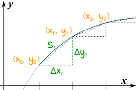
The idea is to increase the number of these segments, while the length of each would become smaller, and consider the sum of the lengths of these segments to approximate the length of a curve. This approximation would be better if all segments are getting smaller, so we can assume that, if there is a limit of the sum of lengths of these segments, if they are infinitesimally small, this limit is, by definition, the length of a curve.
Let's assume that we deal with a motion of a particle along this curve. It's position {x(t), y(t)} is a function of time t and the length covered by this particle during its motion along the curve would be a function of time s(t).
During the time from tn to tn+1a particle moves along the curve from point {x(tn), y(tn)} to {x(tn+1), y(t+11)}.
If all Δtn+1=tn+1−tn are sufficiently small, the length along the curve between each pair of beginning and ending points can be approximated by the length of straight segment between them. The smaller the time intervals - the better is our approximation.
So, it's reasonable to assume that if the time increment is an infinitesimal variable, the difference between exact length along the curve and the length of a straight segment is an infinitesimal of a higher order, which in subsequent summation of all infinitesimals to a total length of a curve would not affect the limit.
Let Δx(tn+1)=x(tn+1)−x(tn) and Δy(tn+1)=y(tn+1)−y(tn).
Then the length of the straight segment between two points on a curve is
Δs(tn)=√Δ²x(tn)+Δ²y(tn)
As customary, with all Δtn converging to zero, we will use an infinitesimal variable dt to designate this increment of a parameter t.
With it, both Δx(tn) and Δy(tn)converge to zero and can be represented by infinitesimal variable increments dx and dy.
Analogously, increment of the length Δs(tn) is an infinitesimal variable ds.
So, the formula for infinitesimal increment of the length of a curve, called a differential along the curve, looks like this:
ds(t) = √[dx(t)]²+[dy(t)]²
As we know, differentials dx(t)and dy(t) can be represented as
dx(t) = x'(t)·dt and
dy(t) = y'(t)·dt
That results in the following representation of a differential along the curve:
ds(t) = √[x'(t)]²+[y'(t)]² ·dt
Connection to Physics
In Physics of motion we know a concept of velocity - a vector with absolute value of a ratio between distance and time (speed), directed towards the direction of motion.
If our motion is not straight forward, but goes along some curve, the direction of motion at any time is along the tangential line to this curve.
If our motion is not constant in speed, we can talk about a very small interval of time during which we can assume the speed changes just a little and calculate an average speed during this time.
Approaching this from a more mathematical viewpoint, we consider a moment of time t, a distance covered by that time as a function s(t) and infinitesimal increment of time dt.
During this infinitesimal time increment of the distance covered would be
s(t+dt) − s(t) = ds(t) =
= √[x'(t)]²+[y'(t)]² ·dt
Then the average speed during this infinitesimal period of time dt equals to
|V(t)| = ds(t)/dt =
= √[x'(t)]²+[y'(t)]²
Derivative x'(t) represents the rate of change of X-coordinate of a particle moving along the curve, derivative y'(t) is the same for Y-coordinate.
What the formula for speed along a curve shows is that velocity of an object moving along a curve, as a vector, can be represented as a sum of two vectors - X-component, a vector directed along the X-axis having value Vx(t)=x(t)=x'(t)and Y-component, a vector directed along the Y-axis having value Vy(t)=y'(t).
In vector form it looks like
V(t) = Vx(t) + Vy(t)
where overline indicates that we deal with vectors and sign + means vector addition. Here V(t) is a velocity vector, Vx(t) is its X-component - projection of velocity onto X-axis and Vy(t)is its Y-component - projection of velocity onto Y-axis.
Tuesday, January 17, 2017
Unizor - Derivatives - Properties of Differential of a Function
Notes to a video lecture on http://www.unizor.com
Properties of Differential
Properties of differential of a function resemble properties of derivative and immediately follow from them.
Below are the proofs of all these properties, using Euler's notation for derivative Dx f(x).
Linear Combination
f(x) = a·g(x) + b·h(x)
df(x) = d(a·g(x) + b·h(x)) =
= Dx(a·g(x) + b·h(x))·dx =
= (a·Dxg(x) + b·Dxh(x))·dx =
= a·Dxg(x)·dx + b·Dxh(x)·dx =
= a·dg(x) + b·dh(x)
Product
f(x) = g(x)·h(x)
df(x) = d(g(x)·h(x)) =
= Dx(g(x)·h(x))·dx =
= (Dxg(x)·h(x) +
+ g(x)·Dxh(x))·dx =
= Dxg(x)·dx·h(x) +
+ g(x)·Dxh(x)·dx =
= dg(x)·h(x)+g(x)·dh(x)
Reciprocal
f(x) = 1/g(x)
df(x) = d(1/g(x)) =
= Dx(1/g(x))·dx =
= −[1/g²(x)]·Dxg(x)·dx =
= −[1/g²(x)]·dg(x)
Compound
f(x) = g(h(x))
df(x) = d(g(h(x))) =
= Dxg(h(x))·dx =
= Dyg(y)·Dxh(x)·dx =
= Dyg(y)·dh(x)
substituting y with h(x).
Let's illustrate this rule for compound functions.
g(x) = sin(x)
h(x) = ln(x)
f(x) = g(h(x)) = sin(ln(x))
First, let's calculate the differential directly by taking a derivative from f(x) and multiplying it by dx.
df(x) = Dx f(x)·dx =
= Dxsin(ln(x))·dx =
using the chain rule of differentiation of a compound function
= cos(ln(x))·(1/x)·dx
On the other hand, let's see what our expression for differential of a compound function gives.
df(x) = d(g(h(x))) =
= Dyg(y)·dh(x) =
= Dysin(y)·dln(x) =
substituting y with ln(x).
= cos(y)·(1/x)·dx =
= cos(ln(x))·(1/x)·dx
As you see, the result is the same as with direct computing the differential.
Implicit
Implicitly defined differential can be calculated using the above rule for differential of a compound function.
Assume, f(x) = g(h(x)) and we need to find dh(x).
Since df(x) = Dyg(y)·dh(x),
we conclude that
dh(x) = df(x)/Dyg(y)
substituting y with h(x).
For example, we need to find dln(x) without the knowledge that
dln(x) = (1/x)·dx
Consider an equality
x = eln(x)
If functions are equal, their differentials at any point are also equal.
dx = deln(x)
Now we can use the expression for a differential of a compound function eln(x) where g(x)=exand h(x)=ln(x).
dx = deln(x) = Dyey·dln(x)
substituting y with ln(x).
Hence,
dx = ey·dln(x) =
= eln(x)·dln(x) = x·dln(x)
Finally,
dln(x) = (1/x)·dx
which corresponds to the result of direct calculations if we use the known expression Dxln(x)=1/x.
Unizor - Derivatives - Concept of Differential
Notes to a video lecture on http://www.unizor.com
Concept of Differential
A concept of differential of a smooth function f(x) at point x=x0 was briefly introduced when we defined a derivative of a function as a linear function of an infinitesimal increment of its argument with a coefficient of proportionality equal to a derivative of this function at point x=x0.
The notation df(x0)/dx=f I(x0), which was introduced when we defined a concept of derivative, reflects this definition.
Here x0 is any point in the domain of function f(x), dx is an infinitesimal increment of argument x from this point and df(x0) is differential of function f(x) introduced above.
The notation that uses d instead of Δ implies that we are not talking about just any particular increment, but about a process of decreasing this increment to zero, thus making it an infinitesimal variable.
Using this type of notation, we can write the definition of a derivative as follows:
f I(x0) =
= limdx→0[f(x0+dx)−f(x0)]/dx
This implies that
[f(x0+dx)−f(x0)]/dx = f I(x0)+ε
where ε is another infinitesimal variable.
Next transformation:
f(x0+dx)−f(x0) =
= f I(x0)·dx+ε·dx
or, using the definition of "littleo" as infinitesimal of higher order,
Δf(x0) = f(x0+Δx)−f(x0) =
= f I(x0)·dx+o(dx) =
= df(x0) + o(dx)
Let me emphasize again that in the above statement dx is not just any increment of argument x, but an infinitesimal variable representing an increment converging to zero.
Similarly, df(x0) is an infinitesimal variable representing an infinitesimal function increment during the process of an increment of an argument converging to zero.
From the definition of a differential
df(x0)=f I(x0)·dx
we see that differential is a function of two arguments: a fixed point x0 within a domain of function f(x) and an infinitesimal increment of an argument dx.
Since x0 is any fixed point, we can talk about a function differential at any value of argument x and use the notation df(x):
df(x)=f I(x)·dx
Here is an illustration of a concept of a differential.
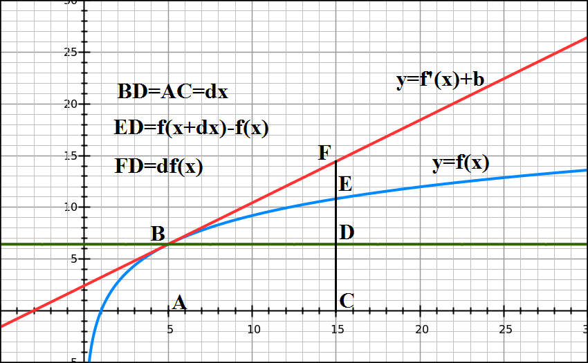
The blue line represents a function, red line - a tangential to it at point A.
Segment BD=AC represents an increment of the argument.
Segment DE is an increment of a function.
Segment DF is function's differential - an increment of a value along the tangential line proportional to the increment of the argument.
When point C moves closer to point A, decreasing the increment of the argument, both segments DE and DF decrease as well, while points E and Fare getting closer to each other, illustrating that increment of a function and its differential are infinitesimals if the increment of the argument is infinitesimal.
What's extremely important is that these two infinitesimals are of the same order as an increment of the argument, while difference between them, segment EF, is an infinitesimal of a higher order.
Recall the Taylor series for function f(x) with expansion center x0:
f(x)=Σn≥0[f (n)(x0)·(x−x0)n/(n!)]
Let's set
dx=x−x0,
Δf(x0)=f(x)−f(x0)
and present this series as follows:
Δf(x0) =
= f I(x0)·dx+f II(x0)·(dx)²/2+...
According to our definition of the differential, this can be expressed as
Δf(x0) = df(x0) + o(dx)
which illustrates the same concept: increment of a function is of the same order as its differential and they differ by an infinitesimal of a higher order than increment of the argument.
It's appropriate to note here that the concept of a differential of a function justifies the Leibniz's notation for a derivative:
f I(x) = df(x)/dx
Conclusion
Differential df(x0) of a function f(x) at some fixed point x0 of its argument is an infinitesimal variable proportional to infinitesimal increment of the argument dx with a coefficient of proportionality equaled to a derivative of this function at chosen point x0:
df(x0) = f I(x0)·dx
Differential differs from increment in a sense that increment is a fixed difference between two values, while differential is an infinitesimal variable.
Thus, Δx is a fixed number that is equal to a difference between the incremented value of argument x=x1 and its base value x=x0:
Δx = x1 − x0
But differential is an infinitesimal variable {x1 − x0} in the process of x1→x0.
As soon as we switch from a fixed Δx to a process by considering Δx→0, increment of an argument Δx becomes its differential dx.
Similarly, Δf(x) is a fixed number that is equal to a difference between the value of a function at incremented value of the argument and the value of a function at the base value of the argument:
Δf(x) = f(x1) − f(x0)
As x1→x0, function increment Δf(x) is getting smaller and relative difference between its values and corresponding values of differential df(x0) are getting smaller as well in a sense that
limΔx→0[Δf(x)]/df(x) = 1
because
limΔx→0[Δf(x)]/Δx = f I(x)
while
df(x)/dx = f I(x)
and dx means the same as Δx→0, that is a process of infinitely decreasing increment of an argument.
Friday, January 13, 2017
Unizor - Derivatives - Problem 2
Notes to a video lecture on http://www.unizor.com
Derivatives - Problems 2
Problem 2.1
Artillery officer needs to choose an angle a cannonball should be launched to reach the maximum distance, provided its linear speed at the moment of launching is fixed.
Assume ideal physical conditions (no air resistance, gravity constant is not changed with the height and whatever else can be assumed to simplify the problem).
Answer
The maximum distance is reached when a cannonball is launched at an angle of π/4=45o
Problem 2.2
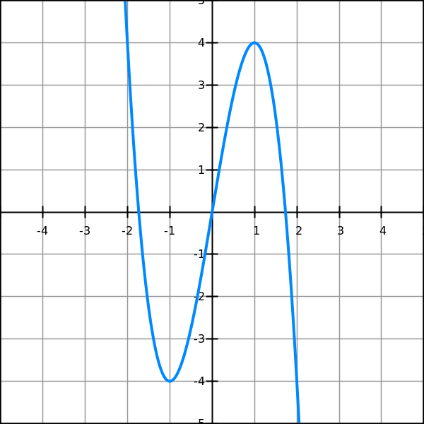
How many zero points does function f(x)=x³−3x+4 have?
Hint
Analyze intervals of monotonic behavior of this function and compare the signs of the function on each interval's ends.
Answer
This function has only one zero point.
Problem 2.3
Consider pulling an object by a rope on a surface with friction. If the rope is horizontal, the force needed to move it with constant speed should be equal to the force of friction. If a rope is at certain angle to horizon, the vertical component of the force applied to it partially neutralizes the friction.
What angle of a rope to horizon is needed to minimize the force applied to it and still to move forward with constant speed?
Consider ideal conditions and a coefficient of friction equal to k.
Answer
The angle or a rope to horizon should be equal to arctan(k).
Solution
Assume, the angle of a rope with horizon is φ (obviously, its range is from 0 to π/2), the weight of an object is P and the force applied to a rope is F.
Then vertical component of the pulling force is
Fv = F·sin(φ)
and horizontal component is
Fh = F·cos(φ)
Vertical component Fv reduces the weight and, therefore, reduces the friction. Therefore, the friction equals to
T = (P−Fv)·k
To pull an object with constant speed this friction force must be equal to horizontal component of the force applied to a rope Fh:
T = Fh
The above equation gives a dependency between the force applied to a rope F and angle of a rope to horizon φ. Having this as a function, we can minimize it and find an optimal angle of minimum force.
Fh = (P−Fv)·k
F·cos(φ) = [P−F·sin(φ)]·k
F·cos(φ)+F·sin(φ)·k = P·k
F = P·k/[cos(φ)+sin(φ)·k]
To minimize this function, let's take its derivative by φ and find where it's equal to zero.
dF/dφ = {−P·k/[cos(φ)+sin(φ)·k]²}·
·[-sin(φ)+cos(φ)·k]
Equation dF/dφ = 0
results in
-sin(φ)+cos(φ)·k = 0
which can be easily solved:
sin(φ) = cos(φ)·k
sin(φ)/cos(φ) = k
tan(φ) = k
φ = arctan(k)
This solution is independent of the weight of an object and means that the greater the friction - the more vertical should be an angle we pull the object to neutralize friction and minimize the force applied to a rope.
If we are talking about practical application of this, when a person pulls something by a rope, for lower friction coefficient we should use longer rope and for higher friction - shorter.
Thursday, January 12, 2017
Unizor - Derivatives - Problem 1
Notes to a video lecture on http://www.unizor.com
Derivatives - Problems 1
Problem 1.1
Consider a sufficiently smooth function f(x).
Is condition f I(x0) = 0
(a) necessary,
(b) sufficient or
(c) necessary and sufficient
for f(x0) to have a local extremum (local maximum or local minimum) at point x=x0?
Prove your answer.
Answer
(a) necessary
It is not sufficient because it might be an inflection point, like for f(x)=x3 at x=0.
Problem 1.2
Consider a sufficiently smooth function f(x).
Is condition f II(x0) = 0
(a) necessary,
(b) sufficient or
(c) necessary and sufficient
for f(x0) to have an inflection point at x=x0?
Prove your answer.
Answer
(a) necessary
It is not sufficient because it might be a point of local extremum, like for f(x)=x4 at x=0.
Problem 1.3 - Derivative of the inverse function theorem
Consider a sufficiently smooth function y=f(x) with derivative
Prove that its inverse y=g(x) (that is, f(g(x))=x) has a derivative
g I(x) = 1 / f I(g(x))
Example 1
y = f(x) = xn
y = g(x) = x1/n (inverse)
f I(x) = n·xn−1
g I(x) = (1/n)·x(1/n)−1 =
= (1/n)·x(1−n)/n
1 / f I(g(x)) = 1 / {n·[x1/n]n−1} =
= (1/n)·1/x(n−1)/n =
= (1/n)·x(1−n)/n = g I(x)
Example 2
y = f(x) = ex
y = g(x) = ln(x) (inverse)
f I(x) = ex
g I(x) = 1/x
1 / f I(g(x)) =
= 1 / e ln(x) = 1/x = g I(x)
Problem 1.4
Consider all possible regular square prisms with a given surface area.
Under what condition between the length of a base' side a and altitude h the volume of this prism will be minimum or maximum?
Solution
Volume V=a²h
Surface area S=2a²+4ah
Since S is given,
h=(S−2a²)/4a
Substitute it into an expression for volume:
V(a) = a²·(S−2a²)/4a =
= (1/4)·a·(S−2a²)
So, we have to find extremum(s) of function
V(a) = (1/4)·a·(S−2a²) =
= (1/4)·(−2a³+S·a)
This is a polynomial function of a, defined on an interval from 0 to a maximum value when the volume is still greater or equal to zero, that is satisfying the condition S−2a² ≥ 0.
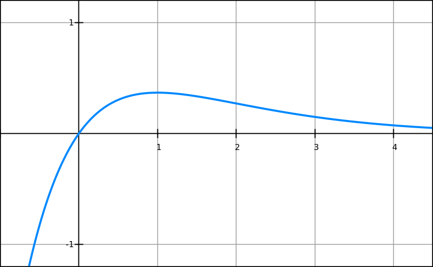
Here is how this function looks on a graph (we have chosen S=6 in this case, so we have to consider this function only on an interval [0,√3]):
As seen from the graph, the extremum of our function within the specified domain is a local maximum.
To find its extremum(s), find the stationary points where derivative equals to zero:
dV/dx = (1/4)·(−6a²+S)
To make sure, we are dealing with a local maximum, we can take a second derivative, it's equal to −3a, and it is negative within a domain of our function, which confirms that a stationary point is a local maximum.
Set the first derivative to 0, getting an equation for variable a:
−6a²+S = 0
Its only root within the established domain is a = √S/6.
Now we can find the corresponding value of altitude h in terms of surface area S:
h = (S−2a²)/4a =
= [S−(S/3)]/(4√S/6) = √S/6.
As we see, h=a, which means that the maximum volume is reached when our prism is a cube.
Unizor - Derivatives - Exercises 2
Notes to a video lecture on http://www.unizor.com
Derivatives - Exercises 2
Exercise 2.1
Given a function f(x)=x·e -x.
Find an equation of a tangential line that touches this function at pointx=2
Answer
y = −e−2·x + 4·e−2
Exercise 2.2
Given a function f(x)=x·e-x.
Find all its maximum, minimum and inflection points.
Answer
f I(x) = e−x·(1−x)
f II(x) = e−x·(x−2)
Point x=1 is a point of local maximum.
Point x=2 is a point of inflection.
There is no point of local minimum.
Exercise 2.3
Given a functionf(x)=sin(x)+cos(x).
Find all intervals where it's monotonically increasing and intervals where it's monotonically decreasing.
Answer
Intervals of monotonic increasing:
[−3π/4+2πn, π/4+2πn]
Intervals of monotonic decreasing:
[π/4+2πn, 5π/4+2πn]
Exercise 2.4
Given a function f(x)=sin(x).
Find all inflection points of this function.
What are the first derivatives at these points?
Answer
x = π·n
First derivatives equal to 1 or −1
Exercise 2.5
Given a function f(x)=x·e-x.
Find an equation of a normal to its graph at point x=2
Answer
y = e2·x + 2·(e−2−e2)
Exercise 2.6
Given a sufficiently smooth function f(x).
Find equations of a tangential line and a normal to its graph at pointx=x0
Answer
Tangential line:
y = f I(x0)·(x−x0) + f(x0)
Normal:
y = −[f I(x0)]−1·(x−x0) + f(x0)
Monday, January 9, 2017
Unizor - Derivatives - Exercises 1
Notes to a video lecture on http://www.unizor.com
Derivatives - Exercises 1
Exercise 1.1
Find derivative of a polynomial
P(x) = Σn∈[0,N] An·xn
Answer
DxP(x) = Σn∈[1,N] An·n·xn−1
Exercise 1.2
As we know,sin(2x)=2sin(x)cos(x)
Find independently derivatives of two functions:
sin(2x), as a compound function g(f(x)), where f(x)=2x and g(x)=sin(x)
and
2sin(x)cos(x) as a product of functions.
Compare the results (supposed to be the same).
Hint
Use an identity
cos(2x)=cos²(x)−sin²(x)
Exercise 1.3
Hyperbolic sine function is defined as
sinh(x) = (ex−e−x)/2
Hyperbolic cosine function is defined as
cosh(x) = (ex+e−x)/2
Prove that
Dxsinh(x) = cosh(x) and
Dxcosh(x) = sinh(x)
which resembles (except the sign in case of derivative of hyperbolic cosine) the situation with regular sine and cosine.
Exercise 1.4
Find derivative of secant and co-secant using their definitions as reciprocal to cosine and sine:
sec(x) = 1 / cos(x) and
csc(x) = 1 / sin(x)
Answer
Dxsec(x) =
= sin(x)/cos²(x) =
= sec(x)tan(x)
Dxcsc(x) =
= −cos(x)/sin²(x) =
= −csc(x)cot(x)
Exercise 1.5
Find derivative of tangent and cotangent functions using their definitions as ratios of sine and cosine:
tan(x) = sin(x) / cos(x) and
cot(x) = cos(x) / sin(x)
Answer
There are different variants, all equivalent:
Dxtan(x) =
= 1+tan²(x) =
= 1/cos²(x) =
= sec²(x)
Dxcot(x) =
= −1−cot²(x) =
= −1/sin²(x) =
= −csc²(x)
Exercise 1.6
Find derivative of arc-sine and arc-cosine using their definitions as inverse functions to sine and cosine:
φ=arcsin(x) ⇒
⇒ −π/2 ≤ φ ≤ π/2; sin(φ)=x
φ=arccos(x) ⇒
⇒ 0 ≤ φ ≤ π; cos(φ)=x
Answer
Dxarcsin(x) = (1−x²)−1/2
Dxarccos(x) = −(1−x²)−1/2
Unizor - Derivatives - Newton's Method of Finding Zeros of a Function
Notes to a video lecture on http://www.unizor.com
Derivatives - Newton's Method
to Find Zeros of Function
The purpose of this lecture is to address a specific problem of finding an approximate solution of equations f(x)=0 using some methodology suggested by Sir Isaac Newton a few centuries ago.
Obviously, it makes sense to apply this methodology when there is no analytical solution of a given equation, or this analytical solution requires too much efforts.
A word of warning should be given up front. This method might sometimes fail to find an approximate solution. After describing this method it will be obvious that under some circumstances the process of finding a solution is not converging to any number.
Let's start with an impractical but illustrative example of a linear function f(x)=2x−4. Obviously, linear equation f(x)=0 looks like 2x−4=0 and can be immediately solved:
2x=4
x=2
But let's approach it differently using the following method.
The graph of f(x)=2x−4 looks like this (blue line):
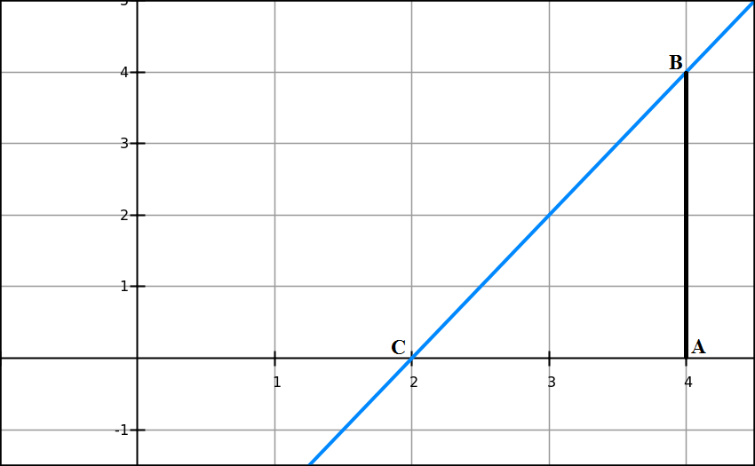
To solve the equation 2x−4=0 means to find the X-coordinate of point C, where the graph intersects the X-axis.
Let's choose any point A with X-coordinate x0 and draw a perpendicular to X-axis from this point to an intersection with the graph of our function f(x)=2x−4 at point B with coordinates {x0, f(x0)} (black line).
We notice that segment AC is a cathetus of triangle ΔABC and, therefore, its length equals to
AC = AB/tan(∠ACB)
We also know that tan(∠ACB)is a derivative of a function f(x)=2x−4 at point C, which is the same as a derivative at any other point, like A, since our function is linear. This derivative is equal to f I(x0)=2.
Therefore, knowing this derivative, X-coordinate of point A, which is equal to x0, and the value of our function at point A, which is equal to f(x0), that is the length of segment AB, we can easily find the length of segment AC and then the X-coordinate of point C:
AC = AB / tan(∠ACB) =
= f(x0) / f I(x0)
Now, X-coordinate of point C, let's call it x1, equals to X-coordinate of point A minus the length of segment AC:
x1 = x0 − f(x0) / f I(x0)
Point A can be taken arbitrarily. Let's say, x0=4.
Then AB=f(x0)=2·4−4=4.
Since tan(∠ACB)=2,AC=4/2=2.
Finally, knowing AC and coordinate of point A (x0=4), we can determine the coordinate of point C:
x1 = x0 − AC = 4−2=2
This is a solution to an original equation 2x−4=0.
Next step towards Newton's Method is to consider a more complex function and how analogous approach to the one above might lead to a solution.
Our next example is a quadratic polynomial
f(x)=(2/9)x²+(2/9)x-(4/9)
presented on the next graph (red line).

We have specifically considered such a function that the linear function described above (blue line) is a tangential line to this new function exactly at a point where we chose to start our calculation x0=4.
Incidentally, it's easy to see that the zero point of this quadratic polynomial is x=1. However, we pretend that we don't know this and attempt to approach this value in a process similar to described above for a linear function.
First of all, note that the behavior of parabola is very smooth on a graph. It is smooth not only in terms of differentiability and continuity of a derivative, but also in terms of its derivative being a monotonic function. In particular, as seen from the graph, direction of parabola and direction of its tangential line at x0=4 (blue line) are very close to each other. From the point of tangency x0=4 both parabola and its tangential line go to zero towards the same direction - to the left from point x0.
The main implication of this is that a zero point C of a tangential line with X-coordinate x1=2, as we calculated above, is closer to a zero point of parabola than original point A at X-coordinate x0=4, where we started the process. Therefore, jumping from point A to point C we got closer to a zero point of a parabola.
An obvious continuation of this process is to recursively repeat the step above, starting at point C with X-coordinate x1=2.
We draw a perpendicular to X-axis at point C to intersection with our parabola at point D with coordinates {x1, f(x1)} and a tangential line to parabola at point D (green line) that intersects X-axis at point E with X-coordinate x2.
Let's determine x2 from triangle ΔEDC similarly to the above procedure:
CE = CD/tan(∠CED)
CD = f(x1) = (2/9)·2²+(2/9)·2−(4/9) = 8/9
tan(∠CED) = f I(x1) =
= (2/9)·2x1+(2/9) = 10/9
CE = (8/9) / (10/9) = 4/5
x2 = x1 − CE =
= x1 − f(x1) / f I(x1) =
= 2−(4/5) = 6/5
Got closer to a zero point of a parabola that we know is x=1, but pretend we don't know it.
Let's repeat this process once more, starting at x2=6/5.
x3 = x2 − f(x2) / f I(x2) ≅
≅ 1.2 − 0.142222 / 0.755556 ≅
≅ 1.01176
Got very close to x=1!
The recursive process described above is the Newton's method of finding arguments where function equals to zero.
Let's formulate it more rigorously.
Assume, we need to find zeros of some smooth function f(x).
Step 0
Start with some approximation of a value of an argument x0that is relatively close to the one where our function equals to zero.
There is no universal recipe for this approximation, but the better your approximation is - the sooner you will approach the real zero of f(x).
And, to be noted, if your starting value is too far from the real zero, the Newton's method might never converge to real zero of our function.
Step 1
From the chosen value x0 calculate the next value of a sequence:
x1 = x0 − f(x0) / f I(x0)
This and subsequent steps are straightforward calculations.
Step 2, 3 etc.
Check two things:
(a) the value of f(xn) - is it close to zero within your chosen precision?
(b) the difference between xn and xn−1 - is it smaller than your chosen precision?
If both checks are satisfactory, stop the process. The last xn is your final result.
If your precision requirements are not satisfied yet, continue.
Repeat the previous step according to this recursive formula:
xn+1 = xn − f(xn) / f I(xn)
As we noted, Newton's method is not universal. A lot depends on properties of function, whose zeros we are trying to find, and on a choice of the first approximation x0.
Let's have an example where Newton's method does not converge to a zero point of a function.
An obvious example is when we choose the first approximation point where a tangential line is parallel to the X-axis.
Thus, in case of a parabola
Another obvious example is an attempt to find a zero point if the function has none. Consider function f(x)=1/x with any starting point. The Newton's method will lead you to infinity.
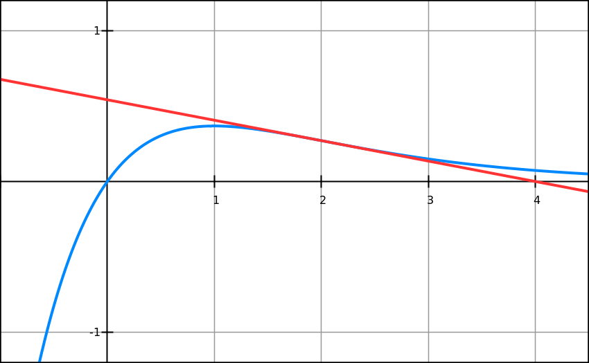
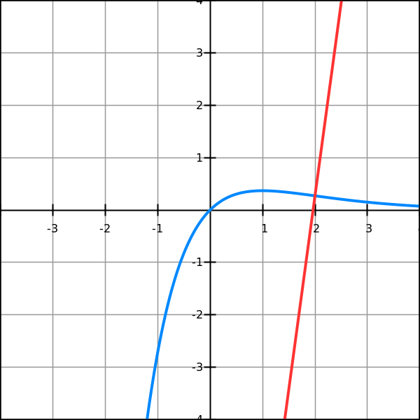
It is very important that the first approximation point should be relatively close to a real zero point of a function. Imagine a function having a zero point and a "hump" near it. If we choose a starting point "behind a hump", the process will never get to a zero point. Here is an example.
f(x)=x·e−x
This function has a maximum at point x=1. At this point the tangential line is parallel to X-axis. If our first approximation x0 is greater or equal to 1, we will never converge to a function's zero point at x=0.
Tuesday, January 3, 2017
Unizor - Calculus - L'Hospital's Rule
Notes to a video lecture on http://www.unizor.com
L'Hopital's Rule
L'Hopital's Rule is a helpful theorem and a related technique to determine certain indeterminate form limits, like 0/0 or ∞/∞.
It should be noted that this theorem has certain limitations that are not always observed and, therefore, the method of determining the indeterminate limit based on L'Hospital's Rule might not always help.
There are, actually, a set of three theorems related to the L'Hospital's Rule, successively more powerful - basic, intermediate and advanced.
Theorem 1
(basic L'Hospital's Rule)
Given two sufficiently smooth functions, F(x) and G(x), defined on some contiguous interval with a point x=x0 inside this interval (which means, x0 belongs to this interval together with its immediate neighborhood).
Assume that F(x0)=G(x0)=0, while G(x), to be able to divide by it, is not equal to zero for
Assume further that the derivative of G(x) at point x=x0is not equal to zero:
G I(x0) ≠ 0
Then
limx→x0 F(x)/G(x) = limx→x0 F I(x)/G I(x) = F I(x0)/G I(x0)
In short, a limit of ratio of two infinitesimal functions equals to a ratio of their derivatives at a limit point.
Analysis
Consider the ratio of two functions depicted on a graph below
F(x)=x²−2x−3 (blue) and
G(x)=−x²+7x−12 (red)
and the limit of their ratio asx→3.
Both functions approach zero asx→3, so their ratio represents an indeterminate form 0/0.
We cannot determine the limit without some clever technique.
In this particular case we can determine the limit using the following method:
F(x) = x²−2x−3 = (x−3)·(x+1)
G(x) = −x²+7x−12 = −(x−3)·(x−4)
F(x)/G(x) = [reducing by (x−3)] = (x+1)/(4−x)
And the limit of this ratio asx→3 equals to
(3+1)/(4−3) = 4
In a more general case this simple method might not work, but we will use these two functions to demonstrate a different method called L'Hospital's Rule.
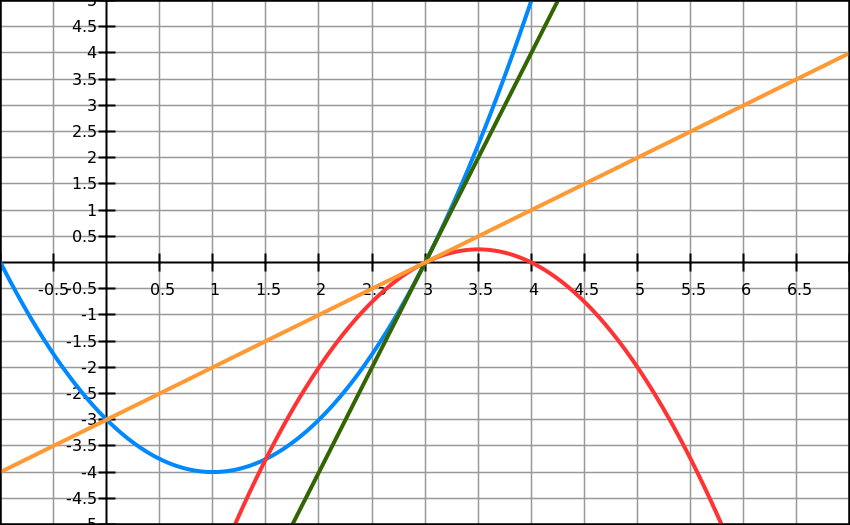
We have drawn two straight lines tangentially to two given functions exactly at point x=3, where we want to find the limit of their ratio:
dark green line is tangential to F(x) and
orange line is tangential to G(x).
In the neighborhood of point of tangency x=3 function and its tangential line are very close to each other. In fact, they are so close that in the ratio of one function over another we can replace the value of a function with the value of the Y-coordinate on the tangential line for the same argument and, as we get closer to a point of tangency, the difference will be an infinitesimal that we can ignore.
And that is the main reason for L'Hospital's Rule.
Here is a justification for this.
Since
[F(x)−F(3)]/(x−3) → F I(3)
the difference between
[F(x)−F(3)]/(x−3) = F I(3) + ε
from which follows
F(x)−F(3) = F I(3)·(x−3) + ε·(x−3)
Recall that F(3) = 0.
Therefore,
F(x) = F I(3)·(x−3) + ε·(x−3)
As x→3, the first member of the sum on the right hand side is an infinitesimal of the same order (this dependency is called Big-O) as x−3 because F I(3) is a constant. The second member is, however, an infinitesimal of a higher order (Little-o) because it's a product of two infinitesimal, ε and x−3.
Similarly,
G(x) = G I(3)·(x−3) + δ·(x−3)
where δ is another infinitesimal.
Using all this, the ratio of our two functions after canceling common multiplier x−3 can be written as
F(x)/G(x) = [F I(3) + ε]/[G I(3) + δ]
Since both ε and δ are infinitesimals, the limit of the expression on the right is
Proof
Since F(x0)=G(x0)=0, we can subtract these from numerator and denominator without changing the value of a ratio.
F(x)/G(x) = [F(x)−F(x0)] / [G(x)−G(x0)]
Now we can divide numerator by x−x0 to obtain an expression that resembles the definition of a derivative for function F(x):
[F(x)−F(x0)]/(x−x0)→F I(x0) as x→x0.
Similarly, we can divide denominator by the same x−x0 to leave the value of a ratio unchanged and to obtain an expression in the denominator that resembles the definition of a derivative for function G(x):
[G(x)−G(x0)]/(x−x0)→G I(x0) as x→x0.
Now the original ratio ofF(x)/G(x) is transformed into this:
F(x)/G(x) = { [F(x)−F(x0)]/(x−x0) } / { [G(x)−G(x0)]/(x−x0) }
Both numerator and denominator of the last expression have limits as x→x0.
They are, correspondingly, derivatives
Therefore, the original limit limx→x0 F(x)/G(x) equals to a ratio of limits, which, in turn, equals to a ratio of two derivatives at point x=x0.
End of proof.
What if the derivative of G(x)at point x0 is equal to zero? We cannot use this basic L'Hospital's Rule. Fortunately, we can extend this theorem to a more general case.
Theorem 2
(general L'Hospital's Rule)
Given two sufficiently smooth functions, F(x) and G(x), defined on segment [a,b].
Assume that F(x)→0 andG(x)→0 as x→+a
(which makes the limit of their ratio indeterminate as x→+a).
Assume further that G I(x) ≠ 0 on segment [a,b] and the limit of the ratio of the derivatives of these functions exists as x→+a.
Then
limx→+a F(x)/G(x) = limx→+a F I(x)/G I(x)
In short, a limit of ratio of two infinitesimal functions equals to a limit of ratio of their derivatives.
NOTE: This theorem does not require existence of derivatives at point x=a or the value of a derivative of G(x) not to be equal to zero at point a. Therefore, we can apply this theorem recursively, going from a ratio of functions to a ratio of their derivatives, then to a ratio of their second derivatives etc. until we get rid of indeterminate form of a limit (or give up).
Proof
Consider any point x∈(a,b) and consider our functions on interval [a,x].
We can apply Cauchy Mean Value Theorem (see the previous lecture) that states that there exists point x0∈[a,x], where the following is true:
F I(x0)/G I(x0) = [F(x)-F(a)]/[G(x)-G(a)] = F(x)/G(x)
Since point x∈(a,b) can be arbitrarily chosen, let's choose x→+a.
Then point x0 would also converge to +a since x0∈[a,x].
That results in
limx→0F I(x0)/G I(x0) = limx→0F(x)/G(x)
(where x0∈[a,x]).
Since we are dealing with sufficiently smooth functions, the last equality is equivalent to
limx→0F I(x)/G I(x) = limx→0F(x)/G(x)
End of proof.
Theorem 3
(extended L'Hospital's Rule)
Not only we can use L'Hospital's Rule to resolve indeterminate form 0/0, but also ∞/∞.
We can also extend the limit point of an argument to ±∞.
Let's prove this for a case of ∞/∞.
Assume, F(x)→∞ and G(x)→∞
as x→a.
Assume that F(x)/G(x)→L
as x→a.
We will prove that
F I(x)/G I(x)→L as well.
Recall that
[1/f(x)] I = −[1/f²(x)]·f I(x).
Therefore,
L = limx→aF(x)/G(x) = limx→a[1/G(x)]/[1/F(x)] =
(now we have 0/0 form, we can apply L'Hospital's Rule)
= limx→a[1/G(x)] I/[1/F(x)] I = limx→a [−1/G(x)]²·G I(x) / [−1/F(x)]²·F I(x) =
= limx→a [F(x)/G(x)]²·limx→aG I(x)/F I(x) = L²·limx→aG I(x)/F I(x)
So, we have obtained an equality
L = L²·limx→aG I(x)/F I(x)
from which follows that
L = limx→aF I(x)/G I(x)
Subscribe to:
Posts (Atom)
