Forced Oscillation 1: UNIZOR.COM - Physics4Teens - Waves - Mechanical Os...

Notes to a video lecture on http://www.unizor.com

Forced Oscillation 1

Oscillation is forced, when some periodic force is applied to an object that can potentially oscillate.

A subject of our analysis will be an object on a spring with no other forces acting on it except one external force that we assume is periodical.

As we know, in the absence of external force the differential equation describing the movement of an object on a spring follows from the Hooke's Law and the Newton's Second Law
m·x"(t) = −k·x(t)
or
m·x"(t) + k·x(t) = 0
with a general solution
x(t) = A·cos(ω₀·t) + B·sin(ω₀·t)
where
A and B are any constants;
ω₀ = √k/m is an inherent natural angular frequency of oscillation of this particular object on this particular spring.

The equation above is homogeneous because, together with any its solution x(t), the function C·x(t) will be a solution as well.

Consider a model of forced oscillation of an object on a spring with a periodic external force acting on it with the following characteristics:
elasticity of a spring k,
mass of an object is m,
force applied to an object is F(t)=F₀·cos(ω·t).

In this lecture we consider a case of angular frequency ω of the periodic external function F(t)=F₀·cos(ω·t) to be different from the inherent natural angular frequency ω₀=√k/m of oscillations without external forces:
ω ≠ ω₀ = √k/m

If external force F(t), described above, is present, the differential equation that describes the oscillation of an object looks like
m·x"(t) = −k·x(t) + F(t)
or, assuming the external force is a periodic function F(t)=F₀·cos(ω·t),
m·x"(t)+ k·x(t) = F₀·cos(ω·t)
The function on the right of this equation makes this equation non-homogeneous.
Our task is to analyze the movement of an object on a spring in the presence of a periodic external function, as described by the above differential equations and initial conditions.

Notice that if some non-homogeneous linear differential equation has two partial solutions x₁(t) and x₂(t), their difference is a partial solution to a corresponding homogeneous linear differential equation.
Indeed, if
m·x₁"(t)+ k·x₁(t) = F₀·cos(ω·t)
and
m·x₂"(t)+ k·x₂(t) = F₀·cos(ω·t)
then for x₃(t)=x₁(t)−x₂(t)
m·x₃"(t)+ k·x₃(t) = 0

From the above observation follows that, in order to find a general solution to a non-homogeneous linear differential equation, it is sufficient to find its one partial solution and add to it a general solution of a corresponding homogeneous equation.

In our case we already know the general solution to a corresponding homogeneous equation
m·x"(t)+ k·x(t) = 0
So, all we need is to find a single partial solution to
m·x"(t)+ k·x(t) = F₀·cos(ω·t)
and add to it the general solution to the above homogeneous equation.

Considering our differential equation, that describes the forced oscillation with a periodic external function, contains function x(t), its second derivative and function cos(ω·t) on its right side, it's reasonable to look for a partial solution x_p(t) in a form of x_p(t)=C·cos(ω·t) and find such a coefficient C that the equation is satisfied.
Then
x_p(t) = C·cos(ω·t)
x'_p(t) = −C·ω·sin(ω·t)
x"_p(t) = −C·ω²·cos(ω·t)
Substituting these into our differential equation, we get
−m·C·ω²·cos(ω·t) +
+ k·C·cos(ω·t) = F₀·cos(ω·t)

Since this is supposed to be true for any time value t, the coefficients at cos(ω·t) must satisfy the equation:
−m·C·ω² + k·C = F₀
from which follows
C = F₀ /(k−m·ω²) =
= F₀ /m·((k/m)−ω²) =
= F₀ / [m·(ω₀²−ω²)]

We have found a partial solution to our non-homogeneous equation:
x_p(t)=F₀·cos(ω·t)/[m·(ω₀²−ω²)]

Now we can express the general solution to a differential equation that describes the forced oscillation by a periodic external function as
x(t)=F₀·cos(ω·t)/[m(ω₀²−ω²)] +
+ A·cos(ω₀·t) + B·sin(ω₀·t)
where
A and B are any constants determined by initial conditions x(0) and x'(0);
ω₀ = √k/m is an inherent natural angular frequency of oscillation of this particular object on this particular spring;
F₀·cos(ω·t) is an external periodic force acting on an object.

It's beneficial to represent A·cos(ω₀·t)+B·sin(ω₀·t) through a single trigonometric function as follows.
Let
D = √A²+B²
Angle φ is defined by
cos(φ) = A/D
sin(φ) = B/D
(on a Cartesian coordinate plane this angle is the one from the X-axis to a vector with coordinates {A,B})
Then
A·cos(ω₀·t)+B·sin(ω₀·t) =
= D·[cos(φ)·cos(ω₀·t) +
+ sin(φ)·sin(ω₀·t)] =
= D·cos(ω₀·t−φ)

Now the general solution to our differential equation that describes forced oscillation looks like
x(t)=F₀·cos(ω·t)/[m(ω₀²−ω²)] +
+ D·cos(ω₀·t−φ)
where
F₀ is an amplitude of a periodic external force;
ω - angular frequency of a periodic external force;
m - mass of an object on a spring;
k - elasticity of a spring;
ω₀=√k/m is an inherent natural angular frequency of oscillation of this particular object on this particular spring;
t is time;
D and φ parameters are determined by initial conditions for x(0) and x'(0).

As you see from the formula for a general solution, it's essential that ω₀≠ω, that is an angular frequency of the external force is not equal to an inherent natural angular frequency of the object and a spring in the absence of external force.
Their equality renders zero in the denominator of a formula, invalidating the whole approach.
What happens if these frequencies are equal is a subject of the next lecture.

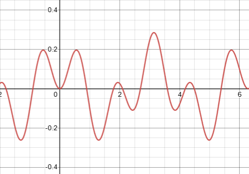
The solution to a forced oscillation in a case of ω₀≠ω represents a superposition of two sinusoidal functions with different frequencies.
Let's represent it graphically for some specific case of initial conditions and parameters.

Initial conditions:
x(0) = 0
x'(0) = 0
From these initial conditions follows
0 = F₀/[m(ω₀²−ω²)] + D·cos(φ)
0 = D·ω₀·sin(φ)
The second equation results in φ=0, from which the first equation gives
D = −F₀/[m(ω₀²−ω²)]
Parameters:
m=1
k=4
ω₀=√k/m=2
F₀=3
ω=5
The parameters above define the value of D:
D=−3/(4−25)=1/7

With the above initial conditions and parameters the oscillation of the object is described by function
x(t)=−3·cos(5t)/21+cos(2t)/7 =
= [cos(2t)−cos(5t)]/7

The graph of this function looks like this

Viscosity Damping 3: UNIZOR.COM - Physics4Teens - Waves - Mechanical Osc...

Notes to a video lecture on http://www.unizor.com

Viscosity Damping 3
Underdamping

This lecture continues analyzing the damped oscillation in a case of underdamping. It relies on equations and symbols presented in the previous two lectures.

The main differential equation that describes the damped oscillation is
m·x"(t) + c·x'(t) + k·x(t) = 0
where
m is a mass of a object attached to a free end of a spring,
c is viscosity of environment surrounding a spring, as it acts against motion of an object,
k is elasticity of a spring,
x(t) is displacement of an object from its neutral position on a spring.
We also consider initial conditions
x(0) = a (initial stretch),
x'(0) = 0 (no initial speed).

In search of two partial solutions of the equation above we used a function
x(t) = e^γ·t
where γ - some (generally, complex) number.
The reason for this is that, substituting this function with its first and second derivatives into the differential equation, we get
x'(t) = γ·e^γ·t
x"(t) = γ²·e^γ·t
and the differential equation is
γ²·m·e^γ·t + γ·c·e^γ·t + k·e^γ·t = 0

Canceling e^γ·t, which never equal to zero, we get a quadratic equation for γ
γ²·m + γ·c + k = 0
with any of its solutions (generally, complex), used in function e^γ·t, delivering the partial solution of the original differential equation.

Case 3

Discriminant of this quadratic equation Δ=c²−4k·m is NEGATIVE

Let
ω² = −Δ /4m² = k/m − (c/(2m))²
where ω - some positive real number.

Then the solution to a quadratic equation for γ above is a set of two complex numbers
γ_1,2 = −c/(2m) ± ω·i
where i²=−1 is an imaginary unit.

Two partial solutions of our differential equation in the domain of complex functions of real argument t are
x₁(t) = e ^{[−c/(2m)+ω·i]·t} and
x₂(t) = e ^{[−c/(2m)−ω·i]·t}

Recall the Euler's formula
e^i·t = cos(t) + i·sin(t)
that you can find in the "Math 4 Teens" course on this site UNIZOR.COM - Math 4 Teens - Trigonometry - Complex Numbers and Trigonometry - Euler's Formula.

Using Euler's formula, we can split two partial solutions of our differential equation into real and imaginary parts:
x₁(t) = x_1.Re(t) + i·x_1.Im(t)
where
x_1.Re(t) = e^−c·t/(2m)·cos(ω·t)
and
x_1.Im(t) = e^−c·t/(2m)·sin(ω·t)
Similarly,
x₂(t) = x_2.Re(t) + i·x_2.Im(t)
where
x_2.Re(t) = e^−c·t/(2m)·cos(−ω·t) =
= e^−c·t/(2m)·cos(ω·t)
and
x_2.Im(t) = e^−c·t/(2m)·sin(−ω·t) =
= e^−c·t/(2m)·sin(ω·t)

If a complex function x(t) satisfies a linear differential equation, its real and imaginary parts must separately satisfy it as well. This obvious statement follows from the fact that, if a(t)+i·b(t)=0 for all t, then a(t)=0 and b(t)=0 for all t.

Therefore, if
x(t) = x_Re(t) + i·x_Im(t)
is a solution of our differential equation, then
x_Re(t) and x_Im(t)
are solutions in their own rights.

Therefore, we have two linearly independent real functions that are partial solutions to our differential equation:
x₁(t) = e^−c·t/(2m)·cos(ω·t)
x₂(t) = e^−c·t/(2m)·sin(ω·t)

Any linear combination of these two functions also is a solution to our differential equation.
This allows to express a general solution as
x(t) = e^−c·t/(2m) ·
· [C₁·cos(ω·t)+C₂·sin(ω·t)]

The expression above for any C₁ and C₂ not simultaneously equal to zero can be simplified as follows.
Let φ be such an angle that
cos(φ) = C₁ /√C₁²+C₂²
sin(φ) = C₂ /√C₁²+C₂²
This angle can easily be constructed, it's an angle from the X-axis to a vector with endpoint at coordinates (C₁,C₂).
Then
x(t) = e^−c·t/(2m)·√C₁²+C₂²·
· [cos(φ)·cos(ω·t) +
+ sin(φ)·sin(ω·t)] =
= e^−c·t/(2m)·√C₁²+C₂² ·
· cos(ω·t−φ) =
= D·e^−c·t/(2m)·cos(ω·t−φ)
where D=√C₁²+C₂² can be any positive real number not equal to zero.
This is a general solution of our differential equation in the case of negative discriminant Δ=c²−4m·k,
where
D - any positive constant
φ - any angle (phase shift)
ω= √−Δ /(2m).

Simple check confirms that this is a solution to our differential equation.

As we see, the motion is a combination of sinusoidal oscillation cos(ω·t−φ) and a damping factor D·e^−c·t/(2m), which reduces the amplitude of oscillation, as the time goes by.
The amplitude of the oscillation is exponentially diminishing.

Let's determine constants D and φ from initial conditions on the position and speed of an object.
At t=0 the position is x(0)=a and speed is x'(0)=0.
x(t) = D·e^−c·t/(2m)·cos(ω·t−φ)
x'(t) = −D·e^−c·t/(2m) ·
· [ω·sin(ω·t−φ) +
+ (c/(2m))·cos(ω·t−φ)]

From this for t=0 follows
D·cos(−φ) = a
−D·[ω·sin(−φ) +
+ (c/(2m))·cos(−φ)] = 0
or
D·cos(φ) = a
D·[−ω·sin(φ) +
+ (c/(2m))·cos(φ)] = 0
or
D·cos(φ) = a
−D·ω·sin(φ) + c·a/(2m) = 0
or
D·cos(φ) = a
D·sin(φ) = c·a/(2m·ω)

From these we can obtain
D² = a²·[1+c²/(4m²·ω²)]
D = a·√1+c²/(4m²·ω²)

For phase φ we can find
cos(φ) =
= 1/√1+c²/(4m²·ω²)
sin(φ) =
= c/[2m·ω·√1+c²/(4m²·ω²)]

Let's calculate the exact expression for this function for some sample values of the constants involved:
a=√3
m=1
c=2
k=4
Δ=c²−4m·k=−12
ω²=−(c/(2m))²+k/m=3
D=a·√1+c²/(4m²·ω²)=2
cos(φ)=
=1/√1+c²/(4m²·ω²)=√3/2
sin(φ)=
=c/2m·ω·√1+c²/(4m²·ω²)=1/2
φ=π/6

Finally, the equation that describes an object's motion
x(t) = D·e^−c·t/(2m)·cos(ω·t−φ)=
= 2·e^−t·cos(√3·t−π/6)

Let's draw a graph of our sample function
x(t) = 2·e^−t·cos(√3·t−π/6)


This graph confirms that the real oscillation does take place in case Δ=c²−4k·m is NEGATIVE, but its amplitude is exponentially diminishes due to damping effect.
The effect of damping of viscous environment is not strong enough to completely suppress the back and forth movement of an object on a spring, but sufficient to make these oscillation less and less significant.
This is called underdamping or small damping.

Viscosity Damping 2: UNIZOR.COM - Physics4Teens - Waves - Mechanical Osc...

Notes to a video lecture on http://www.unizor.com

Viscosity Damping 2
Critical Damping

This lecture continues analyzing the damped oscillation in a case of critical damping. It relies on equations and symbols presented in the previous lecture.

The main differential equation that describes the damped oscillation is
m·x"(t) + c·x'(t) + k·x(t) = 0
where
m is a mass of a object attached to a free end of a spring,
c is viscosity of environment surrounding a spring, as it acts against motion of an object,
k is elasticity of a spring,
x(t) is displacement of an object from its neutral position on a spring.
We also consider initial conditions
x(0) = a (initial stretch),
x'(0) = 0 (no initial speed).

In search of two partial solutions of the equation above we used in a previous lecture a function
x(t) = e^γ·t
where γ - some (generally, complex) number.
The reason for this is that, substituting this function with its first and second derivatives into the differential equation, we get
x'(t) = γ·e^γ·t
x"(t) = γ²·e^γ·t
and the differential equation is
γ²·m·e^γ·t + γ·c·e^γ·t + k·e^γ·t = 0

Canceling e^γ·t, which never equal to zero, we get a quadratic equation for γ
γ²·m + γ·c + k = 0
with any of its solutions (generally, complex), used in function e^γ·t, delivering the solution of the original differential equation.

Case 2
Δ=c²−4k·m EQUALS to ZERO

So, we assume now that the discriminant of the quadratic equation above is zero:
Δ = c²−4k·m = 0.
Then two roots to the quadratic equation above coincide:
γ_1,2 = −c/(2m)

As we see, in this case our approach delivered only one partial solution to our differential equation:
x₁(t) = e^−c·t/(2m)
But, to get to a general solution, we need two partial ones.

The second partial solution we will search among functions x₂(t)=t·e^γ·t.
x'₂(t) = e^γ·t + t·γ·e^γ·t
x"₂(t) = γ·e^γ·t + γ·e^γ·t + t·γ²·e^γ·t
and the differential equation is
m·[γ·e^γ·t + γ·e^γ·t + t·γ²·e^γ·t] +
+ c·[e^γ·t + t·γ·e^γ·t] + k·t·e^γ·t = 0

Canceling exponent e^γ·t that never equals to zero, we obtain
m·[γ + γ + t·γ²] +
+ c·[1 + t·γ] + k·t = 0

Let's group the terms of this equation
t·[m·γ² + c·γ + k] + 2m·γ + c = 0

If we can find such γ that the expression above is always zero for any t, the corresponding function x₂(t)=t·e^γ·t will be a second partial solution we are looking for.

First of all, we should use the fact that the case we are considering now is
Δ = c²−4k·m = 0.
From this follows that
k = c²/(4m)
Substituting this into the above equation, we get
t·[m·γ² + c·γ + c²/(4m)] +
+ 2m·γ + c = 0

Now let's choose such γ that nullifies the part not involved in multiplication by t:
2m·γ + c = 0
γ = −c/(2m)
What it does with a coefficient at t is as follows:
m·γ² + c·γ + c²/(4m) =
= m·c²/(4m²) − c²/(2m) +
+ c²/(4m) =
= c²/(4m) − c²/(2m) +
+ c²/(4m) = 0
So, the coefficient at t is also equals to zero.

Therefore, with γ=−c/(2m) the quadratic equation above is satisfied for any t and function x₂(t)=t·e^−c·t/(2m) is the second partial solution to our differential equations.

Now, having two partial solutions
x₁(t) = e^−c·t/(2m) and
x₂(t) = t·e^−c·t/(2m),
we can formulate a general solution to critically damped oscillation, when Δ=c²−4k·m=0:
x(t) = A·x₁(t) + B·x₂(t) =
= A·e^−c·t/(2m) + B·t·e^−c·t/(2m)

We can determine coefficients A and B from initial conditions
x(0) = a and
x'(0) = 0
From this we get
A = a and
−A·c/(2m) + B = 0

Therefore, our two coefficients are A=a and B=a·c/(2m).
General solution for of a case of critical damping, when c²=4m·k, is
x(t) = a·e^−c·t/(2m) +
+ (a·c/(2m))·t·e^−c·t/(2m) =
= a·(1+c·t/(2m))·e^−c·t/(2m)

Let's calculate the exact expression for this function for some sample values of the constants involved:
a=12
m=1
c=10
k=25
Δ=c²−4m·k=0
x(t) = 12·(1+5t)·e^−5t

Now let's check if this solution satisfies our differential equation
m·x"(t) + c·x'(t) + k·x(t) = 0
Substituting the assumed values for coefficients, it looks like this:
x"(t) + 10·x'(t) + 25·x(t) = 0

Let's check it out for our sample function
x(t) = 12·(1+5t)·e^−5t
x'(t) = 12·5·e^−5t +
+ 12·(1+5t)·(−5)·e^−5t =
= −300t·e^−5t
x"(t) = −300·e^−5t+1500t·e^−5t

Substituting these expressions into equation
x"(t) + 10·x'(t) + 25·x(t) =
= −300·e^−5t+1500t·e^−5t −
− 10·300t·e^−5t +
+ 25·12·(1+5t)·e^−5t =
= −300·e^−5t + 1500t·e^−5t −
− 3000t·e^−5t +
+ 300·e^−5t + 1500t·e^−5t =
= 0 (OK)

Let's check the initial conditions.
x(0)=12=a (OK)
x'(0)=0 (OK)

Let's draw a graph of our sample function
x(t) = 12·(1+5t)·e^−5t


This graph confirms that the displacement of an object from the neutral position monotonically goes to zero, that is it moves in one direction only towards the neutral position without oscillation.
The effect of damping of viscous environment is so strong that it prevents the object to oscillate on a spring.
This was a case of critical damping.

Viscosity Damping 1: UNIZOR.COM - Physics4Teens - Waves - Mechanical Osc...

Notes to a video lecture on http://www.unizor.com

Viscosity Damping 1
Over-Damping

Another variety of damping is related to viscosity of the environment, where oscillation takes place.
An example of this is an oscillation under water.
Each motion of an object on a spring in this case is supposed to overcome a resistance of water that surrounds it.

Interesting distinction of an oscillation under water from previously studied oscillation with friction is that the resistance of water is greater if the speed of an oscillating object is greater, while the friction resistance is constant and depends only on the weight of an object.

This property of the force of resistance to be dependent on (for our theoretical studies to be proportional to) speed is expressed by a formula that is supported by experiments:
F_v(t) = −c·x'(t)
where
t is time parameter;
F_v(t) is the force of resistance caused by viscosity of the environment where oscillation occurs;
x(t) is a displacement of an object from the neutral position on a spring (positive displacement corresponds to stretching, negative - to squeezing a spring);
x'(t) is an object's speed (first derivative of displacement);
c is a damping coefficient that depends on geometrical properties of an object and physical properties of environment, where oscillation takes place.
A minus sign in the formula signifies that the resistance force is opposite to a direction of movement, defined by a sign of a speed.

Equipped by the formula above and by Hooke's Law, describing the force of a spring on an object F_s(t) as being proportional to a displacement of an object from its neutral position on a spring x(t) with coefficient of proportionality k that depends on elasticity of a spring
F_s(t) = −k·x(t)
we come up with a total force F_t(t) acting on an object, oscillating in a viscous environment:
F_t(t) = F_s(t) + F_v(t)

Since the object's acceleration (second derivative of displacement) x"(t) and mass m are related to the total force acting on an object by the Second Newton's Law
F_t(t) = m·x"(t)
we have an equation of motion for an oscillating object in the viscous environment
m·x"(t) = −k·x(t) − c·x'(t)
or
m·x"(t) + c·x'(t) + k·x(t) = 0

This is linear differential equation that we will solve to get the formula for a displacement of an object from its neutral position on a spring x(t) as a function of time.

At this point we'd like to refer you to "Math 4 Teens" course on the same site UNIZOR.COM as this lecture will help to refresh your knowledge about linear differential equations of the second order. From the Unizor home screen choose "Math 4 Teens" - "Calculus" - "Ordinary Differential Equations, Higher Order Equations", where Hooke's Law is presented and general approach to solving linear differential equations of the second order is discussed.

The general solution to a linear differential equation of the second order, like the one above, can be found by finding two functions that satisfy this equation x₁(t) and x₂(t), called partial solutions, and describing the general solution as a linear combination of these two functions
x(t) = A·x₁(t) + B·x₂(t).
The coefficients A and B depend on two initial conditions x(0) and x'(0).

In the lecture about Hooke's Law, as an example of linear differential equation of the second order, it was suggested to seek partial solutions based on function x(t) = e^γ·t
where γ - some (generally, complex) number.
The reason for this is that, substituting this function with its first and second derivatives into the differential equation, we get
x'(t) = γ·e^γ·t
x"(t) = γ²·e^γ·t
and the differential equation is
γ²·m·e^γ·t + γ·c·e^γ·t + k·e^γ·t = 0

Canceling e^γ·t, which never equal to zero, we get a quadratic equation for γ
γ²·m + γ·c + k = 0
with any of its solutions (generally, complex), used in function e^γ·t, delivering the solution of the original differential equation.

Since a quadratic equation has exactly two solutions among complex numbers γ₁ and γ₂, we have two solutions to our original differential equations: x₁(t)=e^γ₁·t and x₂(t)=e^γ₂·t.

Moreover, since the differential equation is linear, any linear combination of the above two solutions will be a solution to a differential equation.
Therefore, the general solution looks like
x(t) = A·e^γ₁·t + B·e^γ₂·t
where constants A and B are defined by two initial conditions of the motion described by our differential equation.

Switching from theory to concrete results for our differential equation presented above, our first task is to solve the quadratic equation to find γ₁ and γ₂
γ²·m + γ·c + k = 0

Very important for a solution to this equation is an expression under radical - discriminant Δ=c²−4k·m.
If it's not negative, both roots of our equation are real, otherwise we have to consider complex roots.

Solutions to this equations are:
γ_1,2 = [−c±√c²−4k·m] /(2m)
or
γ_1,2 = −c/(2m)±√(c/(2m))²−k/m

At this point we will consider three different cases of a discriminant of our quadratic equation:
Δ=c²−4k·m is positive
Δ=c²−4k·m equals to zero
Δ=c²−4k·m is negative
The first case is analyzed in this lecture, two others - in the next.

Case 1
Δ=c²−4k·m is POSITIVE

Let
ω² = Δ /m² = (c/(2m))²−k/m
where ω - some non-negative real number.
Obviously, ω is smaller then c/(2m).
Then the solutions to our equations are
γ_1,2 = −c/(2m) ± ω
Since ω is smaller then c/(2m), both solutions to our quadratic equation are negative.

General solution to our differential equation is
x(t) = A·e^{(−c/(2m)+ω)·t} +
+ B·e^{(−c/(2m)−ω)·t}

Let's determine coefficients A and B from initial conditions on the position and speed of an object.
At t=0 the position is x(0)=a and speed is x'(0)=0.
From this follows
A + B = a
(−c/(2m)+ω)·A +
+ (−c/(2m)−ω)·B = 0 Simplifying the second equation, we get the system of 2 linear equations with two unknowns A and B
A + B = a
−c/(2m)·(A+B) + ω·(A−B) = 0 Using the first equation for A+B=a in the second one, we obtain:
A + B = a
−c·a/(2m) + ω·(A−B) = 0
or
A + B = a
A − B = c·a/(2m·ω)

From these two equations we obtain the values of A and B:
A = a·[1+c/(2m·ω)]/2
B = a·[1−c/(2m·ω)]/2

Solution to our differential equation with given initial conditions is
x(t) = (a/2)·[1+c/(2m·ω)]·
·e^{(−c/(2m)+ω)·t} +
+ (a/2)·[1−c/(2m·ω)]·
·e^{(−c/(2m)−ω)·t}
This function describes the position of an object on a spring at any moment of time t relatively to its neutral position on a spring.

Regardless of the signs of coefficients A and B, both exponents in the above expression for x(t) are negative and each term is monotonously going to zero as time t increases to infinity, so the whole function x(t) that characterizes the displacement of the object on a spring in a viscous environment is decreasing to zero as time t increases to infinity. That is, the object moves towards its neutral position on a spring.

To further investigate the character of object's movement, let's find its speed, as it moves toward the neutral position. It requires to take the derivative of the above function describing its position.
x'(t) = (a/2)·(−c/(2m)+ω)·
·[1+c/(2m·ω)]·e^{(−c/(2m)+ω)·t} +
+ (a/2)·(−c/(2m)−ω)·
·[1−c/(2m·ω)]·e^{(−c/(2m)−ω)·t} =
= (a/2)·e^−c·t/(2m)·
·[(ω−c²/(4ωm²))·e^ωt +
+ (−ω+c²/(4ωm²))·e^−ωt] =
= (a/(8ωm²))·e^−c·t/(2m)·
·[(4ω²m²−c²)·e^ωt +
+ (−4ω²m²+c²)·e^−ωt] =
= (a/(8ωm²))·e^−c·t/(2m)·
·(−4m·k·e^ωt+4m·k·e^−ωt) =
= (a·k/(2ωm))·e^−c·t/(2m)·
·(−e^ωt+e^−ωt)

The expression for x'(t) can only be equal to zero, if e^ωt=e^−ωt,
which possible only if t=0.

Notice that, since ω is a non-negative real number smaller then c/(2m), the absolute value of x'(t) is decreasing to zero as time goes to infinity.
This means that the object's speed never equals to zero after initial moment, our object never stops, never changes the direction and monotonously moves towards its neutral position on a spring, moving slower and slower, as it comes closer to the neutral position.

Let's calculate the exact expression for this function for some sample values of the constants involved:
a=12
m=1
c=10
k=16
Δ=c²−4m·k=36
ω²=(c/(2m))²−k/m=9
ω=3
−c/(2m)+ω=−2
−c/(2m)−ω=−8
A=a·[1+c/(2m·ω)]/2=16
B=a·[1−c/(2m·ω)]/2=−4
x(t) = 16·e^−2t−4·e^−8t

Now let's check if this solution satisfies our differential equation
m·x"(t) + c·x'(t) + k·x(t) = 0
Substituting the assumed values for coefficients, it looks like this:
x"(t) + 10·x'(t) + 16·x(t) = 0

Let's check it out for our sample function
x(t) = 16·e^−2t−4·e^−8t
x'(t) = −32·e^−2t+32·e^−8t
x"(t) = 64·e^−2t−256·e^−8t

Substituting these expressions into equation
x"(t) + 10·x'(t) + 16·x(t) =
= 64·e^−2t−256·e^−8t −
−320·e^−2t+320·e^−8t +
+ 256·e^−2t−64·e^−8t =
= (64−320+256)·e^−2t+
+ (−256+320−64)·e^−8t =
= 0 (OK)

Let's check the initial conditions.
x(0)=16−4=12=a (OK)
x'(0)=−32+32=0 (OK)

Let's draw a graph of our sample function
x(t) = 16·e^−2t−4·e^−8t


This graph confirms that the displacement of an object from the neutral position monotonically goes to zero, that is it moves in one direction only towards the neutral position without oscillation.
The effect of damping of viscous environment is so strong that it prevents the object to oscillate on a spring.
This is called over-damping or large damping.

Friction Damping 2: UNIZOR.COM - Physics4Teens - Waves - Mechanical Osci...

Notes to a video lecture on http://www.unizor.com

Friction Damping 2
Equation of Motion

We continue analyzing the behavior of an object of mass m oscillating on a spring of elasticity k with its oscillation damped by constant force of friction F_f=μ·m·g, where μ is the kinetic friction coefficient and g is the free fall acceleration.

Previous lecture was dealing with energy aspect of this oscillation, and we came to conclusion that on each half a cycle (movement in one particular direction) the amplitude of oscillation is diminishing by 2λ, where λ=μ·m·g/k is the critical distance parameter of an entire oscillating system.

In this lecture we will derive the law of motion - a formula describing the position of an object x(t) as a function of time t.

We assume that initially at time t=t₀=0 a spring is stretched by a distance x(t₀)=a significantly greater than critical distance λ to be able to follow the oscillation for a few cycles of changing the direction of motion.
We further assume, as in previous lectures, that there is no initial push of an object. After stretching the spring to position x(t₀)=a we just let it go by itself. Mathematically, it means that x'(t₀)=0.

For non-damped oscillation, based on the Second Newton's Law and the Hooke's Law, equating the same force acting on an object expressed according to these two laws, we have composed the main differential equation for harmonic oscillation that describes the movement of this object without a friction
m·x"(t) = −k·x(t)
Its solution, considering the initial conditions above, is
x(t) = a·cos(ω·t)
where ω = √k/m

Addition of a constant friction force F_f that acts always against the movement (that is, opposite to a velocity vector) complicates the issue, as it changes the direction after each half a cycle.

Let's consider the first half an oscillation cycle, when an object moves from the initial position x(t₀)=a to a negative direction of coordinate x until it stops at some time t₁ at position x(t₁)=b, which we have determined in the previous lecture to be b=−(a−2λ).

The total force acting on an object is spring's elasticity F_s=−k·x(t) and friction, acting during this first half a cycle in the positive direction and equal to F_f=μ·m·g.
Therefore, the total force acting on an object as it moves from x(t₀)=a to x(t₁)=b is
F = −k·x(t) + μ·m·g

From the Second Newton's Law the same force equals to
F = m·x"(t)
Therefore, we have a differential equation
m·x"(t) = −k·x(t) + μ·m·g
or
x"(t) + (k/m)·x(t) − μ·g = 0
Initial conditions to this differential equation are
x(0) = a
x'(0) = 0

For convenience, we will use variable ω defined as ω²=k/m. It was useful in our discussion of harmonic oscillation and will be helpful here as well.
Then our differential equation looks like
x"(t) + ω²·x(t) − μ·g = 0

Let's try to find a solution using a cos() trigonometric function to satisfy our differential equation:
x(t) = A·cos(ω·t) + B
Then
x'(t) = −A·ω·sin(ω·t)
x"(t) = −A·ω²·cos(ω·t)

Substitute this into our differential equation:
−A·ω²·cos(ω·t) +
+ ω²·[A·cos(ω·t) + B] − μ·g = 0
or
ω²·B = μ·g

From this we find the coefficient B (notice the using of λ, introduced above):
B = μ·g/ω² = μ·g·m/k = λ

The value of coefficient A we can find from the initial condition x(0)=a, where a is an initial stretch of a spring.
x(0) = A·cos(0) + B = A + B
Since x(0)=a and B=λ
a = A + λ
and
A = a − λ

So, the position of our object during its movement from x(t₀=0)=a to x(t₁)=b=−(a−2λ) is
x(t) = (a−λ)·cos(ω·t) + λ

The points where the speed of our object equals to zero are the beginning x(t₀=0)=a and the end x(t₁)=b of its moving in negative direction. As a checking, let's use our equation of motion to find these points.
x'(t) = −(a−λ)·ω·sin(ω·t) = 0
Since we assumed that a is significantly greater than λ, the only case when it's equal to zero is when sin(ω·t)=0, that is ω·t=π·N, where N is any integer number.

The first time (N=0) the speed is zero at the beginning, when t=t₀=0 and an object is in its initial position at distance a from the neutral position.
The next one (N=1) is when ωt=π or t=t₁=π/ω.
Substituting this value for time and using the property cos(π)=−1, we obtain the position where the movement stops
x(t₁) = x(π/ω) =
= (a−λ)·cos(π) + λ =
= 2λ−a =
= −(a−2λ)

This is exactly the same value we obtained by using the energy considerations in the previous lecture - original deviation on stretching a, reduced by 2λ during the first half a cycle, when an object moves towards negative direction, crosses the neutral point (so, its coordinate becomes negative), squeezes a spring until it finally stops.

Let's analyze the second half of the first cycle, when an object moves from most negative position towards positive direction with expanding spring.
The initial position at this time t₁=π/ω is x(t₁)=−(a−2λ) with initial speed x'(t₁)=0.
The differential equation describing the movement is slightly different because the force of friction now is directed towards the negative end of the axis against the direction of the object towards the positive direction.

Combined force of a spring and friction is
F_s + F_f = −k·x(t) − μ·m·g

The differential equation of motion, based on the Newton's Second Law, is
m·x"(t) = −k·x(t) − μ·m·g
or
x"(t) = −(k/m)·x(t) − μ·g

Let's try to find a solution using a cos() trigonometric function to satisfy our differential equation:
x(t) = A·cos(ω·t) + B
Then
x'(t) = −A·ω·sin(ω·t)
x"(t) = −A·ω²·cos(ω·t)

Substitute this into our differential equation:
−A·ω²·cos(ω·t) +
+ ω²·[A·cos(ω·t) + B] + μ·g = 0
or
ω²·B = −μ·g

From this we find the coefficient B (notice the using of λ, introduced above):
B = −μ·g/ω² = −μ·g·m/k = −λ

The value of coefficient A we can find from the initial condition x(t₁)=−(a−2λ), where a is an initial stretch of a spring and t₁=π/ω.
x(t₁) = A·cos(π) + B = −A + B
Since we have an initial condition x(t₁)=−(a−2λ) and B=−λ, the equation for A is
−(a−2λ) = −A − λ
and
A = a − 3λ

Therefore, the equation of motion of an object in the second half of the first cycle is
x(t) = (a−3λ)·cos(ω·t) − λ

Very important characteristic of this motion is that its general behavior is similar to the motion during the first half of the first cycle - based on a cosine function with the same argument ω·t. It means that the time between negative most and positive most positions of an object remains constant and equal to π/ω, while amplitude is diminishing with each half a cycle by 2λ.

The speed of an object x'(t) at the end of the second half of the first cycle is zero. Let's determine the time t₂ when it happens.
x'(t) = −(a−3λ)·ω·sin(ω·t) = 0
Since we assumed that a is significantly greater than λ to assure multiple cycles of an object, this expression equals to 0 when sin(ω·t) = 0, that is ω·t=π·N, where N is any integer.
N=0 corresponded to the initial position of an object at x(t₀)=a,
N=1 corresponded to the position of an object at the end of the first half of the first cycle at x(t₁)=−(a−2λ),
N=2 corresponds to the position of an object at the end of the second half of the first cycle.

With N=2 the time of the end of the second half of the first cycle is
t₂ = 2π/ω
From this we can find the position of an object at the end of the second half of the first cycle:
x(t₂ ) = (a−3λ)·cos(2π) − λ =
= a − 4λ
This corresponds to the results based on energy considerations, obtained in the previous lecture.


Summary

The motion of an object on a spring with constant friction is sinusoidal with constant timing between extreme positive and negative positions relative to the neutral. This timing equals to π/ω, where ω²=k/m - a ratio of a spring's elasticity and object's mass.

The amplitude of oscillations is diminishing on every half cycle by the same constant 2λ, where λ is a critical distance equaled to μ·m·g/k, where μ is the coefficient of kinetic friction.