Monday, October 31, 2016
Unizor - Derivatives - Reciprocal of a Function
Notes to a video lecture on http://www.unizor.com
Derivative Properties -
Reciprocal to a Function
Our purpose is to express the derivative of a reciprocal of a function in terms of its own derivative.
Assume that the real functionf(x) is defined anddifferentiable (that is, its derivative exist) on certain interval with a derivative f I(x).
Let's determine the derivative of its reciprocal
h(x) = 1/f(x) wherever f(x) ≠ 0.
The increment of function h(x)is
Δh(x) = h(x+Δx)−h(x) =
= 1/f(x+Δx) − 1/f(x) =
= [f(x)−f(x+Δx)]/[f(x+Δx)·f(x)]
= −Δf(x)/[f(x+Δx)·f(x)]
Next operations to find a derivative are: dividing the function increment Δh(x) by an increment of an argument Δxand going to a limit as Δx→0.
Δh(x)/Δx =
= [−Δf(x)/Δx)]/[f(x+Δx)·f(x)]
Since function f(x) is differentiable, there is a limit of Δf(x)/Δx as Δx→0. This limit isf I(x).
At the same time
f(x+Δx) → f(x)
as Δx→0.
Recall the properties of limits:
if two sequences have limits Land M, then their product has a limit L·M;
if two sequences have limits Land M ≠ 0, then their ratio has a limit L/M.
Therefore,
Δh(x)/Δx→−f I(x)/f²(x)
Hence,
hI(x) = −f I(x)/f²(x)
It's called the Product Rule of differentiation.
Different forms of notation of this rule are:
(1) [1/f(x)] I = −f I(x)/f²(x)
(2) d[1/f(x)]/dx = −[df(x)/dx]·[1/f²(x)]
Examples
[sec(x)] I = [1/cos(x)] I =
= −[cos(x)] I/cos²(x) =
= sin(x)/cos²(x)
(d/dx)[tan(x)] =
= (d/dx)[sin(x)/cos(x)] =
= (d/dx){[sin(x)]·[1/cos(x)]} =
= (d/dx)[sin(x)]·[1/cos(x)] + sin(x)·(d/dx)[1/cos(x)] =
= cos(x)·[1/cos(x)] + sin(x)·sin(x)/cos²(x) =
= 1+tan²(x)
de−x/dx =
= (d/dx)(1/ex) =
= −[(d/dx)(ex)]/[(ex)²] =
= −ex/[(ex)²] =
= −1/ex =
= −e−x
Dx[f(x)/g(x)] =
= [Dxf(x)]·[1/g(x)] + f(x)·{Dx[1/g(x)]} =
= [Dxf(x)]·[1/g(x)] − f(x)·[Dxg(x)]/g²(x) =
= g(x)·[Dxf(x)]·/g²(x) − f(x)·[Dxg(x)]/g²(x) =
= [g(x)·f I(x)−f(x)·g I(x)]/g²(x)
Unizor - Derivatives - Product of Functions
Notes to a video lecture on http://www.unizor.com
Derivative Properties -
Product of Two Functions
Our purpose is to express the derivative of a product of two functions in terms of derivatives of each of them.
Assume that two real functionsf(x) and g(x) are defined anddifferentiable (that is, their derivatives exist) on certain interval with derivatives, correspondingly, f I(x) and gI(x).
Let's determine the derivative of their product
h(x) = f(x)·g(x)
The increment of function h(x)is
Δh(x) = h(x+Δx)−h(x) =
= [f(x+Δx)·g(x+Δx)] −
− [f(x)·g(x)] =
= [f(x+Δx)·g(x+Δx)] −
− [f(x+Δx)·g(x)] +
+ [f(x+Δx)·g(x)] −
− [f(x)·g(x)] =
= f(x+Δx)·[g(x+Δx)−g(x)] +
+ g(x)·[f(x+Δx)−f(x)] =
= f(x+Δx)·Δg(x) + g(x)·Δf(x)
Next operations to find a derivative are: dividing the function increment Δh(x) by an increment of an argument Δxand going to a limit as Δx→0.
Δh(x)/Δx =
= f(x+Δx)·Δg(x)/Δx +
+ g(x)·Δf(x)/Δx
Since both functions f(x) andg(x) are differentiable, there is a limit of Δf(x)/Δx and Δg(x)/Δxas Δx→0. These limits are, correspondingly, f I(x) and gI(x).
At the same time
f(x+Δx) → f(x)
as Δx→0.
Recall the properties of limits:
if two sequences have limits Land M, then their sum has a limit L+M and their product has a limit L·M.
Therefore,
Δh(x)/Δx→f(x)·gI(x)+g(x)·f I(x)
Hence,
hI(x) = f(x)·gI(x)+g(x)·f I(x)
It's called the Product Rule of differentiation.
Different forms of notation of this rule are:
(1) [f(x)·g(x)] I =
= f I(x)·g(x)+f(x)·gI(x)
(2) d[f(x)·g(x)]/dx =
= f(x)·dg(x)/dx+g(x)·df(x)/dx
Examples
[x³·cos(x)] I =
= 3x²·cos(x)−x³·sin(x)
d(3x³·2x)/dx =
= 3x³·ln(2)·2x+9x²·2x
(d/dx)[sin(2x)] =
= (d/dx)[2sin(x)·cos(x)] =
= 2cos(x)·cos(x)−2sin(x)·sin(x)
= 2[cos²(x)−sin²(x)] =
= 2cos(2x)
Dx[x³·5x·cos(x)] =
= Dx[(x³·5x)·cos(x)] =
= Dx(x³·5x)·cos(x) + (x³·5x)·Dx[cos(x)] =
= Dx(x³)·5x·cos(x) + x³·Dx(5x)·cos(x) + x³·5x·Dx[cos(x)] =
= 3x²·5x·cos(x) + x³·ln(5)·5x·cos(x) − x³·5x·sin(x)
Unizor - Derivatives - Linear Combination of Functions
Notes to a video lecture on http://www.unizor.com
Derivative Properties -
Linear Combination of Functions
Our purpose is to express the derivative of a linear combination of two functions in terms of derivatives of each of them.
Assume that two real functionsf(x) and g(x) are defined anddifferentiable (that is, their derivatives exist) on certain interval with derivatives, correspondingly, f I(x) and
Let's determine the derivative of their linear combination
h(x) = a·f(x)+b·g(x)
where a and b are some real numbers.
The increment of function h(x)is
Δh(x) = h(x+Δx)−h(x) =
= [a·f(x+Δx)+b·g(x+Δx)] −
− [a·f(x)+b·g(x)] =
= a·[f(x+Δx)−f(x)] +
+ b·[g(x+Δx)−g(x)] =
= a·Δf(x)+b·Δg(x)
Next operations to find a derivative are: dividing the function increment Δh(x) by an increment of an argument Δxand going to a limit as Δx→0.
Δh(x)/Δx =
= [a·Δf(x)+b·Δg(x)]/Δx =
= a·Δf(x)/Δx+b·Δg(x)/Δx
Since both functions f(x) andg(x) are differentiable, there is a limit of Δf(x)/Δx and Δg(x)/Δxas Δx→0. These limits are, correspondingly, f I(x) and
Recall the properties of limits:
if a sequence has a limit L, then this sequence multiplied by a constant k has limit k·L;
if two sequences have limits Land M, then their sum has a limit L+M.
Therefore,
a·Δf(x)/Δx → a·f I(x)
b·Δg(x)/Δx → b·gI(x)
and, finally,
Δh(x)/Δx → a·f I(x)+b·gI(x)
Hence,
hI(x) = a·f I(x)+b·gI(x)
In other words, derivative of a linear combination of differentiable functions equals to a similar linear combination of their derivatives.
Different forms of notation of this rule are:
(1) [a·f(x)+b·g(x)] I =
= a·f I(x)+b·gI(x)
(2) d[a·f(x)+b·g(x)]/dx =
= a·df(x)/dx+b·dg(x)/dx
(3) (d/dx)[a·f(x)+b·g(x)] =
= a·(d/dx)f(x)+b·(d/dx)g(x)
(4) Dx[a·f(x)+b·g(x)] =
= a·Dxf(x)+b·Dxg(x)
Examples
[5·sin(x)−7·cos(x)] I =
= 5·cos(x)+7·sin(x)
(d/dx)(2x²−3x) = 4x−3
d(2ex−x)/dx = 2ex−1
Dx[2x²−3ex+4cos(x)] =
= 4x−3ex−4sin(x)
Unizor - Derivatives - Higher Order Derivatives
Notes to a video lecture on http://www.unizor.com
Higher Order Derivatives
We have introduced a concept of derivative at point x0 of a real function f(x) defined in some neighborhood of this point as the following limit (if it exists):
limΔx→0[f(x0+Δx)−f(x)]/Δx
The limit defining a derivative of function f(x) at point x0, if it exists, is some real value defined by both the function itself and a point x0 in its domain.
Therefore, for all these points of a domain of function f(x)where this limit exists the derivative is a new function defined at all these points.
This new function, a derivative of function f(x), defined at all points of a domain of functionf(x) where the above limit exists, is traditionally denoted as f I(x) and called the first derivative of function f(x).
The domain of the derivative
At this point we can consider
Alternative notation for the second derivative is d²f(x)/dx²or d²/dx²(f(x)).
This process of derivation can be continued resulting in thethird derivative of function f(x)denoted as
The next step is the fourth derivative of function f(x)denoted as
Let's illustrate this process with examples.
Example 1
f(x) = a (constant)
etc.
Example 2
f(x) = xn
etc.
Example 3
f(x) = ax
etc.
Example 4
f(x) = sin(x)
etc.
Saturday, October 8, 2016
Unizor - Derivatives - Examples - Trigonometric Functions
Notes to a video lecture on http://www.unizor.com
Derivative Examples -
Trigonometric Functions
1. f(x) = sin(x)
f'(x) = cos(x)
Proof
The function increment is
sin(x+Δx)−sin(x) =
= sin(x)·cos(Δx) +
+ cos(x)·sin(Δx) −
− sin(x) =
= sin(x)·(cos(Δx)−1) +
+ cos(x)·sin(Δx) =
= −sin(x)·2sin²(Δx/2) +
+ cos(x)·sin(Δx)
Now we can use an amazing limit
sin(x)/x→1 as x→0
Based on this,
−sin(x)·2sin²(Δx/2)/Δx → 0 and
cos(x)·sin(Δx)/Δx → cos(x)
The result for a derivative is, therefore,
f'(x) = cos(x)
2. f(x) = cos(x)
f'(x) = −sin(x)
Proof
The function increment is
cos(x+Δx)−cos(x) =
= cos(x)·cos(Δx)−sin(x)·sin(Δx) −
− cos(x) =
= cos(x)·(cos(Δx)−1) −
− sin(x)·sin(Δx) =
= −cos(x)·2sin²(Δx/2) −
− sin(x)·sin(Δx)
Now we can use an amazing limit
sin(x)/x→1 as x→0
Based on this,
−cos(x)·2sin²(Δx/2)/Δx → 0 and
sin(x)·sin(Δx)/Δx → sin(x)
The result for a derivative is, therefore,
f'(x) = −sin(x)
Unizor - Derivatives - Examples - Exponential Functions
Notes to a video lecture on http://www.unizor.com
Derivative Examples -
Exponential Functions
1. f(x) = ex
f'(x) = ex
Proof
Function increment is
ex+Δx − ex =
= ex·(eΔx−1)
Therefore, to find derivative, we have to find a limit of the following expression as Δx→0:
ex·(eΔx−1)/Δx
Since
(eΔx−1)/Δx → 1 as Δx → 0,
the derivative is
f'(x) = ex
2. f(x) = ax
f'(x) = ln(a)·ax
Proof
We will use the identity
a = eln(a)
that follows directly from the definition of the natural logarithm.
The function increment looks now as follows:
ax+Δx − ax =
= ax·(eΔx·ln(a)−1)
Therefore, to find derivative, we have to find a limit of the following expression as Δx→0:
ax·(eΔx·ln(a)−1)/Δx
Obviously,
(eΔx·ln(a)−1)/(Δx·ln(a)) → 1
Therefore,
(eΔx·ln(a)−1)/Δx → ln(a)
from which follows that the derivative equals to
f'(x) = ln(a)·ax
Unizor - Derivatives - Examples - Power Function
Notes to a video lecture on http://www.unizor.com
Derivative Examples -
Power Functions
1. f(x) = xn
f'(x) = n·xn−1
Proof
Using Newton's binomial formula,
(x+Δx)n=xn+n·xn−1·Δx+P·Δ2x
where P is some polynomial of x and Δx.
Therefore,
[(x+Δx)n−xn]/Δx =
= n·xn−1+P·Δx
As Δx→0, this expression tends to n·xn−1
2. f(x) = √x (defined for x ≥ 0)
f'(x) = 1/(2√x)
Notice that derivative does not exist for x=0. So, the domain of a derivative is narrower than the domain of the original function.
Proof
We assume that x takes only positive values.
Let's multiply and divide the expression for function increment √x+Δx − √x
by √x+Δx + √x
Since (a−b)·(a+b)=a²−b², the result will be
Δx/(√x+Δx + √x)
Dividing this by increment of argument Δx and going to the limit as Δx→0, the result will be 1/(2√x)
Unizor - Derivatives - Notation
Notes to a video lecture on http://www.unizor.com
Derivatives - Notation
We have introduced a concept of derivative at point x0 of a real function f(x) defined in some neighborhood of this point as the following limit (if it exists):
limΔx→0[f(x0+Δx)−f(x)]/Δx
Let's emphasize once more that this definition is valid only if the limit above exists.
For some functions, like f(x)=2x this limit exists at any point of their domain. For some others, like f(x)=|x|, there are points (in this case x=0) where this limit does not exist, while at others (x≠0) it does.
The limit defining a derivative of function f(x) at point x0, if it exists, is some real value defined by both the function itself and a point x0 in its domain. Therefore, for all these points of a domain of function f(x) where this limit exists the derivative is a new function defined at all these points.
This new function, a derivative of function f(x), defined at all points of a domain of function f(x) where the above limit exists, is traditionally denoted as f'(x) and called the first derivative of function f(x).
The domain of the derivative f'(x) is a subset of a domain of function f(x) since, in theory, the above limit might not exist at all points of domain of f(x). If this limit exists at each point of domain of f(x), the domain of a derivative f'(x) coincides with the domain of original function f(x).
The definition of a derivative as a limit of ratio of two infinitesimals, increment of function and increment of argument at some point, prompts us to use the following notation:
Δf(x) = f(x+Δx)−f(x)
Then the expression of a derivative of function f(x) at point x would look like this:
f'(x) = limΔx→0Δf(x)/Δx
Using the symbol f' to denote a derivative is attributed to Italian mathematician Lagrange (1736-1813).
To make a notation even shorter, mathematicians have abbreviated the above expression based on limits even further:
f'(x) = df(x)/dx
or, sometimes, (d/dx)f(x).
In these cases expression dx is called a differential of argument x - an infinitesimal variable, and expression df(x) is called a differential of function f(x) - also an infinitesimal variable.
These notations are attributed to German mathematician Leibniz (1646-1716). They are as popular as the Lagrange's notation above. They have certain advantage since they remind us that a derivative is a ratio of two infinitesimals - increment of function df and increment of its argument dx.
In particular, since it implies that these two infinitesimals are proportional to each other with a ratio f'(x) (a function of argument x), it makes sense to use the following notation that relates differentials with a derivative:
df(x) = f'(x)·dx
Newton (England, 1643-1727) used a dot above the function symbol to denote its derivative, which we will rarely use.
Euler used Dx f(x) as a notation of a derivative.
The process of deriving a derivative from a function is called differentiation. We will go through this process for major functions in the Examples.
Wednesday, October 5, 2016
Unizor - Derivatives - Tangential to a Curve
Derivatives - Tangential to Curve
We have defined a derivative as a speed of change of function value relative to a change in its argument.
In this lecture we will interpret this concept of derivative geometrically.
Our purpose is to draw a tangential line to a curve that represents a graph of function f(x).
Let's assume that we have a function f(x) defined on some interval (a,b). Point x0 is inside this interval, that is x0∈(a,b). We have to construct a line tangential to a graph of our function f(x) at point x0.
Since tangential line is supposed to have one common point with a curve at a point of tangency (x0,f(x0), we already have one point our tangential line is supposed to pass through. We need a second parameter to define the tangential line. It can be another point it passes through or an angle it forms with another line. The latter method is preferable and that other line is the X-axis.
To determine the angle our tangential line forms with the X-axis, choose a point x1 within the same interval (a,b) close to point x0 and consider a triangle ΔABC on the picture below.
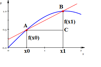
Our plan is to move point x1 closer to x0, which will cause point B to move closer to point A and, therefore, line AB to be closer to a tangential line to a curve at point A.
At any moment of this process we know the tangent of an angle ∠BAC:
tan ∠BAC = BC/AC = [f(x1)−f(x0)] / (x1−x0)
All we have to do now is to take a limit of this expression as point x1 tends to x0. If this limit exists (which for some functions f(x) might not be the case), it will be a tangent of a tangential line to our curve at point A - a second parameter needed to completely define the position of a tangential line at this point.
Traditionally, this is expressed using a substitution
x1 = x0 + Δx
that results in the following expression for tangent of an angle φ formed by a tangential line at point x0 with the X-axis:
tan ∠φ = limΔx→0[f(x0+Δx)−f(x0)]/Δx
As we see, this is exactly the definition of a derivative of a function f(x) at point x0.
Thus, we came to a geometrical interpretation of a derivative - a tangent of an angle formed by a tangential line to a graph of this function with the X-axis.
Tuesday, October 4, 2016
Unizor - Derivatives - Definition
Notes to a video lecture on http://www.unizor.com
Derivatives - Speed of Change
Consider a real function f(x)defined on a set of real numbers and taking real values.
It represents a dependency of some numerical value on certain input parameter. For example, temperature as a function of time or distance the car went as a function of amount of fuel spent, or the force of gravity as a function of an elevation above the surface of the Earth etc.
Let's assume further that this function f(x) is defined on some real interval (a,b) of its argument x, and we are analyzing the function's behavior around a particular point x0 inside this interval. More precisely, we are interested to know how fast the function changes in the neighborhood of this point x0∈(a,b).
Example 1
Back to one of our examples, consider the force of gravity on different levels of elevation. We can measure this force on any level and, comparing these forces G(h0) and G(h1) on two different levels h0 and h1, we can find the average speed of change of gravity on this interval per unit of elevation:
[G(h1)−G(h0)] ∕ (h1−h0)
Notice, this is an average rate of change of the gravity force on interval from h0 to h1, not the rate of change at point h0 we are interested in, because there is a larger space between these two points for this rate to change.
What is also important is that the further points h0 and h1 are from each other - the further our average rate of change is from the one we are interested in. And, the closer point h1 is to h0- the closer our average rate of change of gravity is to the rate at point h0 we need to know.
An obvious solution is to move point h1 as close to h0 as possible.
Mathematical solution is to know the function of gravity force as it depends on the elevation at any elevation level and calculate the limit of the average rate of change as point h1 gets infinitely close to h0:limh1→h0[G(h1)−G(h0)]/(h1−h0)
If this limit exists (and we should not assume it always exists for any function), it can be considered as a true rate of change at point h0.
Example 2
Consider another practical problem
Assume, you are a policeman, who is measuring the speed of the passing cars in order to enforce some speed restrictions in the area.
Assume further that the only tool you have is the stopwatch.
To perform his job, policemen marks two points on the road - A0 and A1 - and, using the stopwatch, measures the time during which any car moves between these points.
Now the average speed on this interval from A0 to A1 will the length of this interval divided by time it took the car to cover it.
But what if the car moved faster than speed limit in the beginning of this interval and slower at the end, so the average speed was below maximum? To detect this, point A1 should be as close to A0 as possible.
Mathematical approach to this problem is as follows.
Let's start with some point on the road as an origin and mark each point with a distance from this origin.
Let's consider a function associated with the movement of a car - exact time t and distance from origin D(t) at each moment in time.
Point A0 was reached at time t0 and its distance from origin is D(t0). Point A1 was reached at time t1 and its distance from origin is D(t1).
The average speed on interval from A0 to A1 can be expressed as
[D(t1)−D(t0)] ∕ (t1−t0)
To get the speed at point A0, we have to know the following limit:
limt1→t0[D(t1)−D(t0)]/(t1−t0)
Example 3
Assume, you are a reporter who has to report the news about the flood. What you need to report is something like this: "At time t0 the level of water was rising with a speed of M meters per hour" (whatever the values of time t0 required).
To accomplish this, you construct the function L(t) of the level of water at each moment in time. Considering you have the value of this function for all moments of time t, you can derive the speed of rising the water at any concrete moment t0 using the following procedure.
You take the level of water at moment t0, which is L(t0), and at some moment t1 after t0, which is L(t1).
The difference between these two levels of water signifies the rising of its level during a period from t0 to t1.
The ratio
[L(t1)−L(t0)] / (t1−t0)
is an average speed of rising water during this period.
If moment t1 is closer to t0, this average speed would represent the speed of rising the waters at moment t0 more precisely, and the closer are these moments - the better would be the evaluation.
Exact speed of rising of the level of water at moment t0 is, therefore
limt1→t0[L(t1)−L(t0)] / (t1−t0)
CONCLUSION
In all the above examples for a given function f(x) we were interested in the speed of its change at some specific value of the argument x0.
This speed of change at x=x0 is defined as
limx1→x0[f(x1)−f(x0)]/(x1−x0)
The limit above, if it exists (which might not be the case) is called a derivative of function f(x) at point x=x0 and denoted as f'(x0).
Since existing of this limit implies its identical value in any trajectory of x1 approaching x0, we can reformulate this using the following formula with identical meaning and notation Δx=x1−x0:
limΔx→0[f(x0+Δx)−f(x0)]/Δx
which is a more traditional definition of derivative of function f(x) at point x=x0.
Subscribe to:
Posts (Atom)
