Unizor - Derivatives - Properties of Function Limits

Notes to a video lecture on http://www.unizor.com


Function Limit - Properties of Limits

Theorem 1

If f(x)→a as x→r, then for any positive A
A·f(x)→A·a as x→r.

Proof

(1a) Using a definition of function limit based on convergence of {f(x_n)} to a for any {x_n}→r, the proof is in the corresponding property of a sequence limit, since {A·f(x_n)}converges to A·a.
Indeed, take any sequence of arguments {x_n} that converges to r.
Since {f(x_n)}→a,
{A·f(x_n)}→A·a by known property of the converging sequences.
So, we have just proven that
∀ {x_n}→r: {A·f(x_n)}→A·a, which corresponds to the first definition of convergence of function A·f(x) to A·a.

(1b) Let's prove this using ε-δdefinition of a function limit.
It's given that
∀ ε>0 ∃ δ>0:
|x−r| ≤ δ ⇒ |f(x)−a| ≤ ε
We have to prove that
∀ ε>0 ∃ δ>0:
|x−r| ≤ δ ⇒ |A·f(x)−A·a| ≤ ε
Using the fact that f(x)→a inε-δ sense, do the following steps.
Step 1 - choose any positive ε.
Step 2 - calculate ε' = ε/A.
Step 3 - using the convergence of f(x), for this ε' find δ such that, if x is withinδ-neighborhood of r, it's true that f(x) is withinε'-neighborhood of a.
Step 4 - we have proven that, as long as x is withinδ-neighborhood of r, it is true that
a−ε' ≤ f(x) ≤ a+ε';
since ε'=ε/A, represent it using original ε as
a−ε/A ≤ f(x) ≤ a+ε/A.
Step 5 - multiply all parts of this inequality by A (it's positive, so signs of inequality are preserved) getting
A·a−ε ≤ A·f(x) ≤ A·a+ε.
This means that A·f(x) is withinε-neighborhood of A·a.
End of proof.

Theorem 2

If f(x)→a as x→r and
g(x)→b as x→r,
then
f(x)+g(x)→a+b as x→r.

Proof

(2a) Using a definition of function limit based on convergence of {f(x_n)} to a and{g(x_n)} to b for any {x_n}→r, the proof is in the corresponding property of a sequence limits, since {f(x_n)+g(x_n)} converges to a+b.

(2b) Let's prove this using ε-δdefinition of a function limit.
Step 1 - choose any positive ε.
Step 2 - calculate ε' = ε/2.
Step 3 - using the convergence of f(x), for this ε' find δ₁ such that, if x is withinδ₁-neighborhood of r, it's true that f(x) is withinε'-neighborhood of a.
Step 4 - using the convergence of g(x), for this ε' find δ₂ such that, if x is withinδ₂-neighborhood of r, it's true that g(x) is withinε'-neighborhood of b.
Step 5 - calculate
δ = min(δ₁, δ₂);
for this δ both statements are true:
f(x) is within ε'-neighborhoodof a and
g(x) is within ε'-neighborhoodof b.
Step 6 - we have proven that, as long as x is withinδ-neighborhood of r, it is true that
a−ε' ≤ f(x) ≤ a+ε' and
b−ε' ≤ g(x) ≤ b+ε';
since ε'=ε/2, represent it using original ε as
a−ε/2 ≤ f(x) ≤ a+ε/2 and.
b−ε/2 ≤ g(x) ≤ b+ε/2;
Step 7 - add these inequalities getting
a+b−ε ≤ f(x)+g(x) ≤ a+b+ε.
This means that f(x)+g(x) is within ε-neighborhood of a+b.
End of proof.

Theorem 3

If f(x)→a as x→r and
g(x)→b as x→r,
then
f(x)·g(x)→a·b as x→r.

Proof

(3a) Using a definition of function limit based on convergence of {f(x_n)} to a and{g(x_n)} to b for any {x_n}→r, the proof is in the corresponding property of a sequence limits, since {f(x_n)·g(x_n)} converges toa·b.

(3b) Let's make some preparations before proving this theorem using ε-δ terminology.
We have to prove that
|f(x)·g(x)−a·b|→0 as x→r.
Recall a known inequality about absolute values:
|A+B| ≤ |A|+|B|.
We will use it in this proof.

Since both our functions have finite limits, their values are sufficiently close to their corresponding limits as long as an argument is sufficiently close to a limit point.
In particular, there is always such δ₁ that |f(x)−a| ≤ 1 for|x−r| ≤ δ₁ and there is always such δ₂ that |g(x)−b| ≤ 1 for|x−r| ≤ δ₂.
Therefore, for|x−r| ≤ δ₃=min(δ₁,δ₂) we can be sure that |f(x)| ≤ |a|+1 and|g(x)| ≤ |b|+1.

Make an invariant transformation with our expression:
|f(x)·g(x)−a·b| =
= |f(x)·g(x)−a·g(x)+a·g(x)−a·b|

The new expression, using the inequality with absolute values mentioned above, is bounded from above as follows:
|f(x)·g(x)−a·g(x)+a·g(x)−a·b|≤
≤|f(x)·g(x)−a·g(x)| +
+ |a·g(x)−a·b| =
= |g(x)|·|f(x)−a|+|a|·|g(x)−b| ≤
≤ (|b|+1)·|f(x)−a|+|a|·|g(x)−b|

After these preparations we are ready to prove the theorem using ε-δ definition of a function limit.
Step 1 - choose any positive ε.
Step 2 - let ε₁ = ε/[2(|b|+1)].
Step 3 - using the convergence of f(x), for this ε₁ find δ₄ such that, if x is withinδ₄-neighborhood of r, it's true that f(x) is withinε₁-neighborhood of a.
Step 4 - let ε₂ = ε/(2|a|).
Step 5 - using the convergence of g(x), for this ε₂ find δ₅ such that, if x is withinδ₅-neighborhood of r, it's true that g(x) is withinε₂-neighborhood of b.
Step 6 - calculate
δ = min(δ₁, δ₂, δ₃, δ₄, δ₅);
for this δ both statements are true:
f(x) is within ε₁-neighborhoodof a and
g(x) is within ε₂-neighborhoodof b.
Step 7 - we have proven that, as long as x is withinδ-neighborhood of r, it is true that
|f(x)−a| ≤ ε₁ and
|g(x)−b| ≤ ε₂;
since ε₁=ε/(|b|+1) and ε₂=ε/|a|,
represent this using original ε as
|f(x)−a| ≤ ε/(|b|+1) and
|g(x)−b| ≤ ε/|a|;
Step 7 - use the above inequalities in the transformed inequality that we have to prove:
|f(x)·g(x)−a·b| ≤
≤ (|b|+1)·ε/[2(|b|+1)] +
+ |a|·ε/(2|a|) = ε
This means that f(x)·g(x) is within ε-neighborhood of a·b.
End of proof.

Theorem 4

If f(x)→a ≠ 0 as x→r
then
1/f(x)→1/a as x→r.

Proof

(4a) Using a definition of function limit based on convergence of {f(x_n)} to a for any {x_n}→r, the proof is in the corresponding property of a sequence limits, since {1/f(x_n)}converges to 1/a.

(4b) Let's prove this using ε-δdefinition of a function limit.
It's given that
∀ ε>0 ∃ δ>0:
|x−r| ≤ δ ⇒ |f(x)−a| ≤ ε
We have to prove that, assuming a ≠ 0,
∀ ε>0 ∃ δ>0:
|x−r| ≤ δ ⇒ |1/f(x)−1/a| ≤ ε

First of all, since a ≠ 0, function values of f(x) are separated from 0 as long as argument x is sufficiently close to a limit point r.
Indeed, take ε = a/2 and find δ₁such that f(x) is inε=a/2-neighborhood of a (that is, a/2 ≤ f(x) ≤ 3a/2) as long as argument x is inδ₁-neighborhood of the limit point r.

Notice now that
|1/f(x)−1/a|=|f(x)−a| / |f(x)|·|a|
Since a/2 ≤ f(x) ≤ 3a/2 in theδ₁-neighborhood of the limit point r, the denominator of the last expression is greater thana²/2.
Therefore,
|1/f(x)−1/a| ≤ 2·|f(x)−a| / a²
Using the fact that f(x)→a inε-δ sense, do the following steps.
Step 1 - choose any positive ε.
Step 2 - calculate ε' = ε·a²/2.
Step 3 - using the convergence of f(x), for this ε' find δ₂ such that, if x is withinδ₂-neighborhood of r, it's true that f(x) is withinε'-neighborhood of a.
Step 4 - set δ = min(δ₁, δ₂).
Step 5 - we have proven that, as long as x is withinδ-neighborhood of r, it is true that
|f(x) − a| ≤ ε' = ε·a²/2.
Step 6 - substitute this into inequality above:
|1/f(x)−1/a| ≤ 2·|f(x)−a| / a² ≤
≤ 2·(ε·a²/2) / a² = ε.

This means that 1/f(x) is withinε-neighborhood of 1/a.
End of proof.

Unizor - Derivatives - Function Limit - Simple Problems

Notes to a video lecture on http://www.unizor.com


Function Limit - Simple Problems

Let's recall two definitions of a limit of function.

Definition 1
Value a is a limit of functionf(x) when its argument xconverges to real number r, if for ANY sequence of argument values {x_n} converging to r the sequence of function values {f(x_n)} converges to a.
Symbolically:
∀{x_n}→r ⇒ {f(x_n}→a

Definition 2
For any positive ε there should be positive δ such that, if x is withinδ-neighborhood of r (that is,|x−r| ≤ δ), then f(x) will be within ε-neighborhood of a(that is, |f(x)−a| ≤ ε).
Symbolically:
∀ ε>0 ∃ δ>0:
|x−r| ≤ δ ⇒ |f(x)−a| ≤ ε

Solving the problems below, you can use any of these definitions to prove the existence of a limit and to find its concrete value.

Problem 1

Consider a function defined for all real arguments x:
f(x) = Ax
(where A ≠ 0).
Prove that this function has a limit for x→0 and that this limit equals to 0.

Solution 

Let's use Definition 1 above. Consider ANY sequence {x_n}converging to 0.
We will prove that corresponding sequence of function values {f(x_n)=Ax_n}converges to 0 as well.
From {x_n}→0 follows that
∀ε>0 ∃N: n ≥ N ⇒ |x_n| ≤ ε
The above statement is given.
What we have to prove is that
∀ε>0 ∃M: n ≥ M ⇒ |Ax_n| ≤ ε
We can prove the existence of such M for any ε by direct constructing it following these steps:
(a) choose ANY positive ε;
(b) calculate new ε' = ε/|A|;
(c) since {x_n} converging to 0, for this ε' find M such that, ifn ≥ M, then |x_n| ≤ ε';
From |x_n| ≤ ε' follows that|Ax_n| ≤ |A|ε' = ε.
So, for ANY sequence {x_n}converging to 0 and ANY positive ε we have found Msuch that, if n ≥ M, then|Ax_n| ≤ ε.
That means that functionf(x)=Ax converges to 0 as its argument x converges to 0.
End of proof.

Problem 2

Consider a function defined for all real arguments x:
f(x) = x²
Prove that this function has a limit for x→0 and that this limit equals to 0.

Solution 

Let's use Definition 1 above. Consider ANY sequence {x_n}converging to 0.
We will prove that corresponding sequence of function values {f(x_n)=x²_n}converges to 0 as well.
From {x_n}→0 follows that
∀ε>0 ∃N: n ≥ N ⇒ |x_n| ≤ ε
The above statement is given.
What we have to prove is that
∀ε>0 ∃M: n ≥ M ⇒ |x²_n| ≤ ε
We can prove the existence of such M for any ε by direct constructing it following these steps:
(a) choose ANY positive ε;
(b) calculate new ε' = ε^1/2;
(c) since {x_n} converging to 0, for this ε' find M such that, ifn ≥ M, then |x_n| ≤ ε';
From |x_n| ≤ ε' follows that|x²_n| ≤ (ε')² = ε.
So, for ANY sequence {x_n}converging to 0 and ANY positive ε we have found Msuch that, if n ≥ M, then|x²_n| ≤ ε.
That means that functionf(x)=x² converges to 0 as its argument x converges to 0.
End of proof.

Problem 3

Consider a function defined for all positive arguments x:
f(x) = log₂(x)
Prove that this function has a limit for x→1 and that this limit equals to 0.

Solution 

Let's use Definition 2 above. Consider ANY positive ε.
We will prove that there is suchδ that, as long as x is withinδ-neighborhood of value 1, function values f(x)=log₂(x)will be within ε-neighborhoodof value 0.
Basically, we have to prove that the inequality |log₂(x)| ≤ εfollows from |x−1| ≤ δ for someδ.
The inequality |log₂(x)| ≤ ε can be represented as
−ε ≤ log₂(x) ≤ ε
If this inequality is true, raising2 to the power of its components will produce an equivalent inequality, since power function 2^x is monotonically increasing.
So, an equivalent inequality is
2^−ε ≤ 2^log₂(x) ≤ 2^ε
or, considering that 2^log₂(x) = x,2^−ε ≤ x ≤ 2^ε.
We can say now that, as long as2^−ε ≤ x ≤ 2^ε, it is true that−ε ≤ log₂(x) ≤ ε and, equivalently, |log₂(x)| ≤ ε.
Let's examine this inequality forx: 2^−ε ≤ x ≤ 2^ε.
We are considering positive ε to be as small as possible. That results in 2^ε to be slightly greater than 1, while 2^−ε to be slightly less then 1. So, an interval (2^−ε,2^ε) encompasses the value of 1 from both sides.
Let's chooseδ=min(1−2^−ε, 2^ε−1).
Now interval (1−δ, 1+δ) is inside a bigger interval (2^−ε,2^ε), while still encompassing the value 1.
Therefore, for anyx∈(1−δ, 1+δ) (this isδ-neighborhood of 1) it is true that −ε ≤ log₂(x) ≤ ε (that isε-neighborhood of 0).
Our problem is solved, for any given ε we have found corresponding δ such that, if xis in δ-neighborhood of 1, it is true that f(x)=log₂(x) is inε-neighborhood of 0.
That means that functionf(x)=log₂(x) converges to 0 as its argument x converges to 1.
End of proof.

Unizor - Derivatives - Equivalence of Function Limit Definitions

Notes to a video lecture on http://www.unizor.com


Function Limit - Why Two Definitions?

Recall two definitions of function limit presented in the previous lecture.

Definition 1

Value a is a limit of functionf(x) when its argument xconverges to real number r, if for ANY sequence of argument values {x_n} converging to r the sequence of function values {f(x_n)} converges to a.

Symbolically:
∀{x_n}→r ⇒ {f(x_n}→a

Definition 2

Value a is a limit of functionf(x) when its argument xconverges to real number r, if for any positive ε there should be positive δ such that, if x is within δ-neighborhood of r(that is, |x−r| ≤ δ), then f(x)will be within ε-neighborhood of a (that is, |f(x)−a| ≤ ε).

Symbolically:
∀ ε>0 ∃ δ>0:
|x−r| ≤ δ ⇒ |f(x)−a| ≤ ε

Sometimes the last two inequalities in the above definition are specified as "less" instead of "less or equal". It makes no difference.

First of all, let's answer the question of the title of this lecture: Why two definitions?

Obviously, there were historical reasons. Mathematicians of 18th and early 19th centuries suggested different approaches to function limits and functioncontinuity that led to both definitions. Cauchy, Bolzano Weierstrass and others contributed to these definitions.
The Definition 1 seems to sound "more human", it seems more natural, though difficult to deal with if we want to prove the existence of a limit.
The Definition 2, seemingly "less human", is easier to use when proving the existence of a limit. It is more constructive.

In this lecture we will prove the equivalence of both definitions. That is, if function has a limit according to Definition 1, it is the same limit according to Definition 2 and, inversely, from existence of a limit by Definition 2 follows that this same limit complies with Definition 1.

Theorem 1
IF
for any sequence of argument values {x_n} converging to r the sequence of function values{f(x_n)} converges to a
[that is, if f(x)→a as x→raccording to Definition 1],
THEN
for any positive ε there should be positive δ such that, if x is within δ-neighborhood of r(symbolically, |x−r| ≤ δ), thenf(x) will be withinε-neighborhood of a(symbolically, |f(x)−a| ≤ ε)
[that is, it follows that f(x)→awhile x→r, according to Definition 2].

Proof

Choose any positive ε, however small, thereby fixing someε-neighborhood around limit value a.
Let's prove an existence of δsuch that, if x is closer to r thanδ, then f(x) will be closer to athan ε.
Assume the opposite, that is, no matter what δ we choose, there is some value of argument x in the δ-neighborhood of r such that f(x) is outside ofε-neighborhood of a.

Let's choose δ₁=1 and find the argument value x₁ such that|x₁−r| ≤ δ₁, while |f(x) is outside of ε-neighborhood of a.
Next choose δ₂=1/2 and find the argument value x₂ such that|x₂−r| ≤ δ₂, while |f(x) is outside of ε-neighborhood of a.
Next choose δ₃=1/3 and find the argument value x₃ such that|x₃−r| ≤ δ₃, while |f(x) is outside of ε-neighborhood of a.
etc.
Generally, on the n^th step choose δ_n=1/n and find the argument value x_n such that|x_n−r| ≤ δ_n, while |f(x) is outside of ε-neighborhood of a.

Continue this process of building sequence {x_n}.
This sequence, obviously, converges to r since|x_n−r| ≤ 1/n, but f(x_n) is always outside of ε-neighborhood of a, that is {f(x_n)} is not converging to a, which contradicts our premise that, as long as {x_n}converges to r, {f(x_n)} must converge to a.

So, our assumption that, no matter what δ we choose, there is some value of argument x in the δ-neighborhood of r such that f(x) is outside of ε-neighborhood of a, is incorrect and there exists such δ that, as soon as argument x is in theδ-neighborhood of r, value of function f(x) is withinε-neighborhood of a.
End of proof.

Theorem 2
IF
for any positive ε there is positive δ such that, if x is within δ-neighborhood of r(symbolically, |x−r| ≤ δ), thenf(x) will be withinε-neighborhood of a(symbolically, |f(x)−a| ≤ ε)
[that is, if f(x)→a as x→raccording to Definition 2],
THEN
for any sequence of argument values {x_n} converging to r the sequence of function values{f(x_n)} converges to a
[that is, it follows that f(x)→awhile x→r, according to Definition 1].

Proof

Let's consider any sequence{x_n}→r and prove that{f(x_n)}→a.
In other words, for any positiveε we will find such number Nthat for all n ≥ N the inequality|f(x_n)−a| ≤ ε is true.

Based on the premise of this theorem, there exists positive δsuch that, if |x−r| ≤ δ, it is true that |f(x)−a| ≤ ε.

Since {x_n}→r, for any δ there exist number N such that, ifn ≥ N, it is true that |x_n−r| ≤ δ.
So, for this particular N it is true that |f(x_n)−a| ≤ ε.
End of proof.

Unizor - Derivatives - Function Limit Definition

Notes to a video lecture on http://www.unizor.com


Function Limit -
Two Definition

A sequence {X_n} from the functional viewpoint can be considered as a function from the set of all natural numbers N(domain of this function) into a set of all real numbers R (co-domain of this function).

Order number n is an argumentof this function, while X_nrepresents a value of this function for argument n.

When we consider a limit of asequence, we have in mind a process of increasing the argument n without any bounds (to infinity, as we might say) and observing the convergence or not convergence of the values X_n to some real number, which in case of convergence is called the limit of this sequenceas order number n increases toinfinity.

More rigorously, real numbera is a limit of a sequence {X_n}, if for any (however small) ε > 0 there exists order number Nsuch that
|a - X_n| ≤ ε for any n ≥ N.

In this lecture we will expand our field from sequences to functions of any real argument and real values. We will generalize the concept of a limit to a process of an argument not only increasing to infinity, but converging to any real number.
After this we will be ready to define derivatives and other interesting principles of Calculus.

To consider a function instead of a sequence presents no efforts, since a sequence is a function. All we do is expanding a domain from all natural numbers N to all real numbers R.

Without much efforts we can define a limit of a function as its argument increases to infinity. This practically repeats the definition of a limit of a sequence and looks like this.

Real number a is a limit of function f(x) when x increases to infinity, if for any positive distance ε, however small, there is a real number r such that for all x ≥ r it is true thatf(x) is closer to a than distance ε, that is |f(x)−a| ≤ ε.

Let's express this symbolically.
∀ ε>0 ∃ r: x ≥ r ⇒ |f(x)−a| ≤ ε

Having a set of natural numbersN as a domain dictates only one type of process where we can observe the change of sequence values - when order number nincreases to infinity.
With a domain expanded to all real numbers we have more choices. One such way, as defined above, is to increase an argument of a function to infinity - total analogy with sequences. Another is to decrease the argument to negative infinity.
Here is how it can be defined.

Real number a is a limit of function f(x) when x decreases to negative infinity, if for any positive distance ε, however small, there is a real number rsuch that for all x ≤ r it is true that f(x) is closer to a than distance ε, that is |f(x)−a| ≤ ε.

Let's express this symbolically.
∀ ε>0 ∃ r: x ≤ r ⇒ |f(x)−a| ≤ ε

Our final expansion of a limit of sequence to limit of function is to define a limit of function when its argument gets closer and closer (converges) to some real number instead of going to positive or negative infinity.

First of all, we have to define this process of convergence of an argument to some real number more precisely.
Obvious choice is to measure the distance between an argument x and some real number r our argument, supposedly, approaches. So, if xis changing from x₁ to x₂, tox₃... to x_n etc. such that sequence {|x_n−r|} isinfinitesimal (that is converges to zero), we can say that xconverges to r.

It is very important to understand that argument x can converge to value r in many different ways forming different infinitesimals. For example, sequence x_n = r+1/n is one such way. Another is x_n = r·(1+1/n). Yet another is x_n = r·2^1/n.
Even more sophisticated way to converge is for x to approach ronly on rational numbers skipping irrationals or, inversely, only on irrational numbers, skipping rationals.
As you see, convergence of an argument to a specific value can be arranged in many different ways, but in any way the distance |x−r| must be infinitesimal, that is must converge to zero.

Let's examine now the behavior of a function f(x) as its argument x converges to valuer. It is natural to assume that function f(x) converges to valuea when its argument xconverges to value r if |f(x)−a|is an infinitesimal when |x−r| is infinitesimal.
Symbolically, we can describe this as
{x_n}→r ⇒ {f(x_n)}→a

It is very important to understand that there might be cases when x converges to r in some way (that is, sequence{|x_n−r|} is infinitesimal) and corresponding sequence of function values f(x_n) converges to a, but, if argument xconverges to r in some other way, function values f(x_n) do not converge to a.
Here is an interesting example. Consider a function f(x) that takes value 0 for all rational arguments x and takes value 1for all irrational x. Now let xapproach point r=0 stepping only on rational numbers likex_n=1/n. All values of f(x_n) will be 0 and we could say that f(x)converges to 0 as x converges to 0. But if we step only on irrational numbers like x_n=π/n, our function will take valuesf(x_n) equaled to 1 and we would assume that f(x) converges to 1as x converges to 0. This does not seem right.

It is appropriate then to formulate the concept of limit in terms of sequences as follows.
Value a is a limit of functionf(x) when its argument xconverges to real number r, if for ANY sequence of argument values {x_n} converging to r the sequence of function values {f(x_n)} converges to a.

Symbolically:
∀{x_n}→r: {f(x_n}→a

Though logically we have come up with a correct definition of a limit of function when its argument converges to a specific real number, it is not easy to verify that concrete function has a concrete limit when its argument converges to concrete real number. We cannot possibly examine ALL the ways an argument approaches its target.
Let's come up with another (equivalent) definition of a limit that can be used to constructively prove statements about limits.

Again, we will use analogy with sequence limits.
The key point to a definition of a limit for a sequence was that, when order number n is sufficiently large (non-mathematically, we can say "sufficiently close to infinity"), the values of sequence members are sufficiently close to its assumed limit. The degree of order number to be "sufficiently close to infinity" (that is, sufficiently large, greater than some number) depends on how close we want our sequence to be to its limit. Greater closeness of a sequence to its limit necessitates larger order number, that is its greater "closeness to infinity", so to speak.

For function limits we will approach more constructive definition analogously. If we assume that some real number ais a limit of a function f(x) as xconverges to r, then for any degree of closeness between a function and its limit there should be a neighborhood of value r in which (that is, if x is within this neighborhood) this degree of closeness between a function and its limit is observed. Greater closeness requires a narrower neighborhood.

Expressing it more precisely, for any positive ε there should be positive δ such that, if x is within δ-neighborhood of r(that is, |x−r| ≤ δ), then f(x) will be within ε-neighborhood of a(that is, |f(x)−a| ≤ ε).

Symbolically:
∀ ε>0 ∃ δ>0:
|x−r| ≤ δ ⇒ |f(x)−a| ≤ ε

Sometimes the last two inequalities in the above definition are specified as "less" instead of "less or equal". It makes no difference.

Unizor - Derivatives - Limit of Ratio of Polynomials

Notes to a video lecture on http://www.unizor.com


Sequence Limit -
Ratio of Polynomials

When a sequence is represented by a ratio of two polynomials of order number n, it's easy to find its limit.
It's all about the members of the highest power in numerator and denominator.

Assume, a sequence is given by an expression
X_n = P(n) / Q(n)
where P(n) is a polynomial of power p (here p - some natural number) of n and Q(n) is a polynomial of power q (here q - some natural number) of n.

So, we can write the following expressions for our polynomials:
P(n) = a₀n^p+a₁n^p−1+...+a_pn⁰
(where a₀ ≠ 0)
Q(n) = b₀n^q+b₁n^q−1+...+b_qn⁰
(where b₀ ≠ 0)

In order to determine the limit of their ratio, let's transform them as follows:
P(n)=n^p(a₀+a₁n⁻¹+...+a_pn^−p)
Q(n)=n^q(b₀+b₁n⁻¹+...+b_pn^−q)

Consider two expressions in parenthesis:
R(n) = a₀+a₁n⁻¹+...+a_pn^−p
S(n) = b₀+b₁n⁻¹+...+b_pn^−q

As order number n increases to infinity, each member of these expressions, except the first (a₀ and b₀) is an infinitesimal and, therefore, has its limit equal to0. Since there is only finite number of these infinitesimals in each expression, the limit of the first one is a₀ and the limit of the second one is b₀.
That means that the limit of their ratio is a₀ / b₀, that is
R(n) / S(n) → a₀ / b₀.

Let's return back to our original ratio of two polynomials.
P(n) / Q(n) =
= [n^p·R(n)] / [n^q·S(n)] =
= n^p−q·[R(n) / S(n)]

Ratio [R(n) / S(n)] has a limit a₀ / b₀ and, therefore, is bounded.
Expression n^p−q is either
infinitesimal (for p less than q) or
constant 1 (for p equaled to q) or
infinitely growing (for p greater than q)

Therefore, the ratio of original polynomials P(n) / Q(n) is a sequence that
(a) is infinitesimal
if p is less than q
(b) converges to a limit a₀ / b₀
if p equals to q
(c) is infinitely growing
if p is greater than q

We have reduced a problem for the limit of a ratio of two polynomials to a simple comparing their highest powers (p and q) and corresponding coefficients at the members in these powers (a₀ and b₀).

We can easily expand this approach to a ratio of two functions that can be represented as a sum of finite number of power functions, like
X_n = U(n) / V(n)
where
U(n) = Σu_i·n^p_i (0 ≤ i ≤ M)
and
V(n) = Σv_i·n^q_j (0 ≤ j ≤ N)

In the above expressions powers p_i and q_j can be any real numbers, not necessarily natural (like 0.5 for a square root or even irrational powers like π).

All we have to do now is position all members of U(n) in order of decreasing of their powers, same with V(n), and factor out that highest power. Remaining members (analogous to R(n) and S(n)above) will contain only members with negative powers, except the first constants (u₀ and v₀ correspondingly), and they all will converge.

Therefore, assuming our functions U(n) and V(n) are already written in the order of decreasing powers of their members, the following expression would correctly represent our ratio
U(n) / V(n) = n^p₀−q₀·W(n)
where p₀ is the highest power among members of U(n), q₀ is the highest power among members of V(n), W(n) is a sequence converging to u₀ / v₀- a ratio of coefficients at the highest powers of functions U(n) and V(n).

Hence, we can make a judgment about convergence of our ratio U(n) / V(n).
(a) it is infinitesimal
if p₀ (the highest power of U(n)) is less than q₀ (the highest power of V(n))
(b) converges to a limit a₀ / b₀
if p₀ equals to q₀
(c) is infinitely growing
if p₀ is greater than q₀.

Unizor - Derivatives - Indeterminate Forms

Notes to a video lecture on http://www.unizor.com


Sequence Limit -
Indeterminate Forms

When a sequence is represented by a short simple formula of the order number n, like {1/n²}, it's easy to find its limit.

When a sequence is a simple operation (sum or product) on other sequences with known or easily obtainable limits, like
{[1+1/(n+1)]+[2/(n+2)]},
it's easy too - just perform the operation on corresponding limits.

The problem arises when we cannot break a sequence into individual components, determine a limit for each component and do the required operations on the limits. Here are a few simple examples:
(a) X_n = (1/n)·(2n+3)
here 1/n is infinitesimal and 2n+3 is infinitely growing, their product is undefined.
(b) X_n = (2n+3)/n
here both numerator and denominator are infinitely growing with undefined limit (you may say that limit is infinity, but it's not a number, so you cannot perform an operation of division anyway)
(c) X_n = sin(n)/n²
here numerator is not even a convergent sequence, while denominator is infinitely growing.

In all cases where we cannot simply determine the limit of a complex sequence as a result of a few operations on the limits of the components, we deal with indeterminate forms.
Each such case should be dealt in some way, very specific for each given sequence, to transform the sequence into equivalent, but easier to deal with form.

Let's consider different cases we might have using concrete example of sequences.

1. Ratio of two infinitesimals
(indeterminate of type 0/0)

(a) (2⁻⁽ⁿ⁺¹⁾+3⁻ⁿ)/2⁻ⁿ =
= 2⁻¹+(3/2)⁻ⁿ → 1/2

(b) sin²(1/n) / [1−cos(1/n)] =
= sin²(1/n)·[1+cos(1/n)] /
/ [1−cos²(1/n)] =
= 1+cos(1/n) → 2

2. Product of infinitesimal and infinitely growing sequence
(indeterminate of type 0·∞)

(a) [1/(n+1)]·n² =
= (n−1)(n+1)/(n+1)+1/(n+1) =
= n−1+1/(n+1)
which is an infinitely growing sequence

(b) n·sin(1/n) =
= sin(1/n) / (1/n) → 1
see lecture Trigonometry - Trigonometric Identities and Equations - Geometry with Trigonometry - Lim sin(x)/x, where it was proven that the limit of sin(x)/x as x→0 equals to 1.

3. Ratio of two infinitely growing sequences
(indeterminate of type ∞/∞)

(a) (n²+n−2)/(2n²+3n−5) =
= [(n+2)(n−)]/[(2n+5)(n−1)] =
= (n+2)/(2n+5) =
= [(2n+5)−1]/[2(2n+5)] =
= 1/2 − 1/[2(2n+5)] → 1/2

(b) [n²·sin(1/n)+1]/n =
= n·sin(1/n)+1/n =
= sin(1/n)/(1/n)+1/n → 1

4. Difference of two infinitely growing sequences
(indeterminate of type ∞−∞)

(a) √(n²+n)−n =
= n / [√(n²+n)+n] =
= n / [n√(1+1/n)+n] =
= 1 / [√(1+1/n)+1] → 1/2

(b) n+1−log₂(2ⁿ−1) =
= 1+log₂[2ⁿ/(2ⁿ−1)] =
= 1+log₂[1+1/(2ⁿ−1)] → 1

CONCLUSION
Many indeterminate forms do have a limit, but, to find it, it's necessary to transform the original sequence into equivalent without indeterminate components.

Unizor - Derivatives - Infinity

Notes to a video lecture on http://www.unizor.com


Sequence Limit - Infinity

We use the term infinity rather casually, understanding that this is a large, very large, larger than anything quantity.
This lecture is about a concept of infinity as it is understood by mathematicians.

First of all, let's agree that there is no such number or such quantity as infinity in classical math. There are some advanced parts of higher levels of math, where infinity is introduced as a concrete object, but it is beyond the scope of this course. So, for our purposes infinity is not a number or quantity. What is it then?

It is a short form of specifying the directional and limitless behavior of a sequence.

Consider a sequence {X_n} that grows boundlessly. That is, for any, however large, number Aexists an order number N such that all members of this sequence with order numbers not less than N are not less than number A.
Using symbols ∀ ("for all" or "for any") and ∃ ("exist"), this can be symbolically written as follows:
∀ A ∃ N: n ≥ N ⇒ X_n ≥ A

For any sequence that behaves in this manner we may say thatit's limit is infinity.
Sometimes we add a characteristic "positive" to a word infinity, if it helps to better understand the behavior of a sequence and to differentiate it from negative infinity described below.
So, the expression about infinity(or positive infinity) being a limit of some sequence cannot be considered absolutely rigorous and it just means that the sequence is boundlessly grows in a sense described above. It would be better to use the term infinitely growing sequence than mentioning the word "limit" for such cases. Also not advisable to use the term "convergent" for these sequences, this is reserved for sequences convergent to real numbers.
Example of such infinitely growing sequence:
{X_n = 2ⁿ}

Similarly, we can introduce a sequence that boundlessly "grows" (in a sense of absolute value, while being negative) to a negative infinity.
The description of this property is analogous to a case withpositive infinity.
If for any negative number A, however large by absolute value, exists an order number Nsuch that all members of this sequence with order numbers not less than N are not greater than number A, we say that the limit of this sequence isnegative infinity.
Symbolically, it can be written as
∀ A ∃ N: n ≥ N ⇒ X_n ≤ A
(notice, we don't have to specify that A is negative since we use "for any" symbol, which includes all negative numbers as well as positive)
Example of such sequence:
{X_n = log₂(1/n)} = {−log₂(n)}

So, terms infinity, positive infinity (same as infinity) andnegative infinity are legitimate mathematical characteristics of sequences that either, being positive starting at some number, grow boundlessly or, while negative after some number, grow by absolute value boundlessly.
Using these terms implies the properties described in detail above. That's why these terms can be considered as a short description of these properties. It's easier and no less rigorous to state "a sequence grows toinfinity" instead of "for any, however large, number A exists an order number N such that all members of this sequence with order numbers not less than Nare not less than number A".
Both expressions mean the same and can be used interchangeably. The former is just a lot shorter and quicker to understand. So is an expression "an infinitely growing sequence".

Examples:
1. X_n = (n²+1)/n
Let's prove that this sequence is limitlessly increasing to infinity.
Choose any boundary numberA, however large. Expression(n²+1)/n=n+1/n is monotonically increasing with an increase of n because, as nincreases by 1, 1/n decreases by a fraction of 1. Therefore, once it grows above A, it will stay above A. So, we just have to find the first member of this sequence that is above A.
Let's find natural order numberN in our sequence for a chosen boundary A by solving the inequality
(n²+1)/n ≥ A
which is equivalent to (since nis positive)
n²−An+1 ≥ 0
Expression
n²−An+1
is a quadratic polynomial of nwith discriminant A²−4, which is positive for large A (any value greater than 2).
This quadratic polynomial limitlessly grows with its argument n.
For any large number A there are two solutions to a quadratic equation n²−An+1 = 0:
n₁ = (A−√A²−4)/2 and
n₂ = (A+√A²−4)/2
For any N greater or equal to a larger of these two solutions n₂the inequality we need will be true.
Therefore, for any number A, however large, the members of our sequence {(n²+1)/n} will be greater or equal to this A as long as the order number n is greater than or equal to
(A+√A²−4)/2.
This proves that this sequence is limitlessly increasing toinfinity.

2. X_n = tan(−πn/[2(n+1)])
Let's prove that this sequence is limitlessly decreasing tonegative infinity.
Choose any boundary numberA, negative and however large by absolute value.
Let's find N for a chosen boundary - number A - by solving the inequality
tan(−πn/[2(n+1)]) ≤ A
which is equivalent to (sincetan(−φ) = −tan(φ))
−tan(πn/[2(n+1)]) ≤ A
or
tan(πn/[2(n+1)]) ≥ −A
Here −A is a positive number, however large, function tan is monotonically increasing on interval [0,π/2).
Expression πn/[2(n+1)] is monotonically increasing to π/2and its tangent is monotonically increasing to infinity as n is increasing. So, all we have to find is such n that
tan(πn/[2(n+1)]) = −A,
which happens at
πn/[2(n+1)] = arctan(−A)
or
πn = 2(n+1)arctan(−A)
From the above equation follows:
n(π−2arctan(−A)) =
= 2arctan(−A)
Therefore,
n = 2arctan(−A) /
/ (π−2arctan(−A))
Since n is a natural number, we have to choose the next natural number greater than the above expression.

3. X_n = n·sin(n)
This sequence is growing by absolute value, but changing the sign from positive to negative and back with the periodicity of2π
That means, the sequence cannot be qualified as having aninfinity (positive or negative) as a limit.
It's not infinitely growing topositive infinity, nor infinitely decreasing to negative infinity.

Unizor - Derivatives - Infinitesimals

Notes to a video lecture on http://www.unizor.com


Sequence Limit - Infinitesimal
(infinitely small)

Special role in mathematics in general and, in particular, in calculus is played by sequences that converge to zero.
These sequences have a special name - infinitesimal. More descriptive name might beinfinitely small.

It is very important to understand that here we are not dealing with any concrete, however small, number, but with a sequence converging to zero.

When we say that ε is an infinitesimal value, we mean that it represents a sequence of values converging to zero, that is a process, a variable that changes its value, gradually getting closer and closer to zero.

When we say that a distance between two objects is an infinitesimal, we imply that these objects are moving towards each other such that the distance between them converges to zero.

When we say that the speed of an object changes by an infinitesimal value during infinitesimal time interval, we mean the following process:
(a) we fix some moment in timeT₀ and the speed of an object at this moment V₀;
(b) we consider an infinite sequence of time intervals starting at T₀ and ending at T₁,T₂,...T_n... such that the difference in time |T_n − T₀|converges to zero as index nincreases;
(c) we measure a speed V_n of an object at each end of intervalT_n;
(d) the difference between the original speed V₀ and the speed at each end of interval V_n is a sequence that converges to zero:
|V_n − V₀| → 0

Properties of infinitesimals are direct consequences of properties of the limits in general:

1. If ε is an infinitesimal (more precisely, if a sequence {ε_n}converges to zero, but we will use the former expression for brevity), then K·ε is also an infinitesimal, where K - any real constant, positive, negative or zero.

2. If ε and δ are two infinitesimals, their sum ε+δ is an infinitesimal as well.

3. If ε and δ are two infinitesimals, their product ε·δis an infinitesimal as well.

Lots of problems are related to a division of one infinitesimal by another, provided the infinitesimal in the denominator does not take the value of zero. The result of this operation can be a sequence that might or might not converge at all and, if it converges, it can converge to any number.
Here are a few examples.

A) ε = {13/n}→0;
δ = {37/n}→0;
⇒ ε/δ = {13n/37n} = {13/37}.
Since sequence ε/δ is a constant, its limit is the same constant, that is 13/37.
Obviously, we can similarly construct two sequences with ratio converging to any number.

B) ε = {13/n}→0;
δ = {37n/(n²+1)}→0;
⇒ ε/δ = {[13(n²+1)]/37n²} =
= {(13/37)·[1+1/(n²+1)]} =
= {(13/37)+13/[37(n²+1)]} =
= 13/37 + γ → 13/37,
since γ is an infinitesimal {13/[37(n²+1)]}→0.

C) ε = {13/n²}→0;
δ = {37n/(n²+1)}→0;
⇒ ε/δ = {[13(n²+1)]/37n³} =
= {(13/37)·[1/n+1/(n²+1)]} =
= {13/(37n)+13/[37(n²+1)]} =
= γ₁ + γ₂ → 0,
since both γ₁=13/(37n) andγ₂=13/[37(n²+1)] are infinitesimals.

D) ε = {13/n}→0;
δ = {37/(n²+1)}→0;
⇒ ε/δ = {[13(n²+1)]/(37n)} =
= (13n)/37+13/(37n)
The last expression is growing limitlessly as n is increasing.
So, the result is not a convergent sequence. However, it is reasonable to say that this sequence "grows to positive infinity" as n increases.
We will discuss a concept of infinity later.

E) ε = {1/n}→0;
δ = {(−1)ⁿ/n}→0;
⇒ ε/δ = {(−1)ⁿ}
The last expression represents a sequence that alternatively takes only two values, 1 and −1. It is not converging to any number, nor can we say that it grows to infinity.

As we see, a ratio of two infinitesimals might be convergent or not-convergent sequence, bounded or unbounded.
If we suspect that it should converge to some limit, we have to resolve this by some transformation into an expression without division between two infinitesimals.

It should be noted, however, that the most interesting cases in dealing with infinitesimals occur exactly at the point of division of one by another. Numerous examples of this can be found in physics (like a concept of speed, where we divide an infinitesimal distance by infinitesimal time interval during which this distance is covered), analysis of smooth functions (like in determining their local maximums and minimums) and many others.

Unizor - Derivatives - Limit of Sequence - Definition and Properties

Notes to a video lecture on http://www.unizor.com


Sequence Limit -
Definition and Properties

Please refer to lectures on sequence limits in the "Limits" chapter of Algebra subject of this course.
Here is a brief reminder of a definition and basic properties of sequence limits.

A sequence S={a_n} is an infinite countable ordered set of real numbers, where for each natural number n exists one and only one element of this set a_n.

Real number L is a limit of a sequence {a_n}, if for any (however small) ε > 0 there exists order number N such that
|L - a_n| ≤ ε for any n ≥ N.

The requirement of existence of an order number N with corresponding sequence term being closer to a limit than any chosen distance ε, however small we choose it, assures that elements of a sequence eventually become, as we say, infinitely close to a limit.
The requirement of absolute value of a distance between limit L and elements of a sequence a_n to be not greater than ε for any n ≥ N assures that, once a sequence get sufficiently close to a limit, it will stay not farther from it.

A sequence that has a limit is called convergent, it converges to its limit.

Let's address some simple properties of limits. All of them were proven in the lectures about sequence limit in the Algebra subject of this course. We strongly recommend to review these proofs in that lecture.

Theorem 1
A convergent sequence is bounded, that is there are two numbers, lower and upper bounds, such that all elements of this sequence are not less than lower and not greater than upper bound.
Symbolically,
{a_n}→L
⇒ ∃ A, B ∀ n: A ≤ a_n ≤ B

Theorem 2
A convergent sequence, multiplied by a factor, converges to a limit that is equal to a limit of an original sequence, multiplied by this factor.
Symbolically,
{a_n}→L
⇒ {K·a_n}→K·L

Theorem 3
A sum of two convergent sequences converges to a limit that is equal to a sum of the limits of these two sequences.
Symbolically,
{a_n}→L; {b_n}→M
⇒ {a_n+b_n}→L+M

Theorem 4
A product of two convergent sequences converges to a limit that is equal to a product of limits of these two sequences.
Symbolically,
{a_n}→L; {b_n}→M
⇒ {a_n·b_n}→L·M

Theorem 5
An inverse of a convergent sequence, that has a non-zero limit, converges to a limit that is equal to an inverse of its limit.
Symbolically,
{a_n}→L; L≠0
⇒ {1/a_n}→1/L

Theorem 6
A ratio of two convergent sequences converges to a limit that is equal to a ratio of limits of these two sequences, provided the limit of denominator is not zero.
Symbolically,
{a_n}→L; {b_n}→M; M≠0
⇒ {a_n/b_n}→L/M

Here are examples of simple sequences that have limits:
{1/n}→0
{(n+1)/n}→1
{(12n²+3n)/(5n²−5)}→12/5

Unizor - Statistics - Normality Test Example

Notes to a video lecture on http://www.unizor.com


Normality Test - Example

As an example of an analysis on normality of statistical distribution consider the hourly sea level observed at Midway Island during a period from January 1st, 2012 to December 31st, 2014.
Raw data are taken from the official Web site Sea Level Center of University of Hawaii.

Based on these data certain analitical calculations were performed and are presented atSea Level at Midway Island 2012-2014 Analysis. The histogram as a picture is at Sea Level at Midway Island 2012-2014 Histogram.

The calculated statistical values are:
minimum 660 mm,
maximum 1859 mm,
average μ = 1125 mm and
standard deviation σ = 142 mm.
We also calculated the double and triple standard deviation.

We have built a histogram of sea level distribution by dividing the range of values into 30 bins and presenting frequencies for each bin in numerical and graphical (histogram) form. The histogram does resemble the bell curve, which is a good indication of normality.

Next we calculated how many data elements fall in σ, 2σ and3σ intervals around the mean values and the results are as follows.
Out of a total of 26304 data elements
26223 (99.69%) fall within 3σinterval around mean value μ,
25265 (96,05%) fall within 2σinterval around mean value μ,
17651 (67.10%) fall within σinterval around mean value μ.
These calculations correspond to theoretical numbers (99.7%, 95% and 68%) for Normal distribution quite well.

The bottom line - the distribution does correspond to Normal.

Unizor - Statistics - Normality Test Methods

Notes to a video lecture on http://www.unizor.com


Normality Test - Methods

In many statistical researches people use criteria that are characteristics of Normal distribution, like the "rule of2σ", assuming that their statistical data do have Normal distribution. But is it always so?

A lot of processes we analyze statistically are extremely complex and random variables observed are really a result of many factors dependently and independently affecting the final result.

Here we resort to Theory of Probabilities and the Central Limit Theorem that states that a sum of random variables under very broad conditions tends to be distributed closer and closer to Normal distribution with the number of components increasing.

Take, for example, a body temperature of a healthy person. It's different for different people and at different times. The cause for a particular temperature is extremely complicated and is the result of work of all the cells in human body, each working at its own regime. All these trillions of cells emit heat and together they determine the body temperature.

This is a perfect case when a sum of many random variables, of which we know very little, results in relatively narrow range of temperature of a body. According to Central Limit Theorem we expect the body temperature to behave like Normally distributed random variable and state that somewhere around 37^oC (or 98.6^oF) lies the average normal temperature of a human body with certain deviation within the range of normality.

Obviously, before applying criteria applicable only to Normal distribution, we have to make sure that statistical data are indeed taken from Normally distributed random variable.
We will discuss a couple of methods that can easily be used to check this hypothesis of Normality.

Using Histograms

The first method is purely visual, but requires the construction of a histogram of distribution.
Let's assume that we have sufficient amount of data to make our histogram representative for the distribution of probabilities of a random variable we observe. Then a histogram of Normal distribution based on these data should resemble familiar bell-shaped curve. Obviously, it cannot be exactly along the ideal bell-shaped curve, but clearly visible numerous deviations from the bell-shaped curve would indicate that an observed random variable is not Normally distributed.

The typical characteristics of a bell-shaped curve are:
(a) symmetry relative to vertical line in the middle between minimum and maximum values;
(b) single maximum in the middle;
(c) visible "hump" (concave downward) in the middle;
(d) gradual change to concave upwards as we move to the left and to the right from the middle.

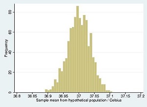
Here is an example of a bell-shaped histogram of a healthy temperature of human body in^oC:


There are a couple of deviations from the ideal bell-shaped curve, but they can be attributed to exceptions and random deviations that always occur in statistical data. Generally speaking, the curve does have a bell shape.

As an opposite example of statistics of a not Normal random variable, consider a distribution of household income in the US. Most likely, the smaller numbers (poor and middle class) will be much more numerous than larger numbers (rich). So, the histogram will be much "heavier" in the smaller numbers, which indicates a not Normal distribution of probabilities.
Here is a histogram for 2010.


So, just looking at a histogram can convey information about whether the observed random variable is Normally distributed or not.

Counting Frequencies

In many cases we use the properties of Normal distribution of a random variable ξ to evaluate the probabilities of its deviation from its mean value μ:
P{|ξ−μ| ≤ σ} ≅ 0.68
P{|ξ−μ| ≤ 2σ} ≅ 0.95
P{|ξ−μ| ≤ 3σ} ≅ 0.997
where σ is standard deviation of Normally distributed random variable ξ.

This can be used as a test of Normality of statistical distribution based on accumulated sample data.
Having the values our random variable took, we can calculate its sample mean μ and sample standard deviation σ. Then we can calculate the ratio of the number of times values of our random variable fall within σ-boundary around sample meanμ, within 2σ-boundary and within 3σ boundary.
If these ratios are far from, correspondingly, 0.68, 0.95 and0.997, the distribution is unlikely Normal.
Obviously, the more data we have - the better correspondence with the above frequencies we should observe for truly Normal variables.

Unizor - Statistics - Correlation Problem 3

Notes to a video lecture on http://www.unizor.com


Statistical Correlation -
Problems 3

To establish the usefulness of a new vaccine, the following statistical data were collected.
Out of 2000 people 1000 randomly chosen people were inoculated with a vaccine and the other 1000 received placebo.
There were 50 cases of illness related to this virus among inoculated and 300 among people who received placebo.
Does this vaccine work?

Solution

Let's put our information into a table.

	Sick	Not Sick	Total
Vaccine	50	950	1000
Placebo	300	700	1000
Total	350	1650	2000

Consider a random variable ξtaking values 1 and 0 for each person depending on whether this person was inoculated (ξ=1) or not (ξ=0). Since 1000 randomly chosen people out of 2000 were inoculated, the probability of ξ to take value 1 is 1000/2000=0.5 and probability of it to take value 0 is the same 0.5.

Consider a random variable ηtaking values 1 and 0 for each person depending on whether this person got sick (η=1) or not (ξ=0). Since 350 people out of 2000 got sick, the probability of η to take value 1 is350/2000=0.175 and probability of it to take value 0 is 1−0.175=0.825.

If vaccine does not help to resist a virus, inoculation random variable ξ and getting sick random variable η are supposed to be independentrandom variables and their correlation should be equal to 0. If vaccine works well, correlation should be negative since vaccination (ξ=1) and sickness (η=1) are opposite to each other.
In any case, it's interesting to find out the value of statistical correlation.

E(ξ·η) =
= 1·50/2000+0·950/20000+
+0·300/2000+0·700/20000 =
=0.025

E(ξ) =
= 1·0.5 + 0·0.5 =
= 0.5

Var(ξ) =
= (1−0.5)²·0.5 + (0−0.5)²·0.5 =
= 0.25

E(η) =
= 1·0.175 + 0·0.825 =
= 0.175

Var(η) =
= (1−0.175)²·0.175 +
+ (0−0.175)²·0.825 =
= 0.144375

Cov(ξ,η) =
= E(ξ·η)−E(ξ)·E(η) =
= 0.025−0.5·0.175 =
= −0.0625

R(ξ,η) =
= Cov(ξ,η)/√Var(ξ)·Var(η) =
= -0.0625/√0.25·0.144375 ≅
≅ −0.328976

As we see, the non-zero correlation exist. It is noticeable but not a very strong correlation, and it is negative, which means that increased value of one random variable is related to decreased value of another, that is vaccination is correlated to not getting sick and non-vaccination correlates with getting sick, as expected.

Consider now two extreme cases.

Case A

If the number of sick people in the vaccinated group is proportional to a number of sick people among whole observed population, we should assume that vaccine has no affect and random variables ξ that reflects inoculation of a person and ηthat reflects his health status are independent. Let's determine what should the number of inoculated sick people x should be: x/1000 = 350/2000
x = 175.
The table of results looks now as

	Sick	Not Sick	Total
Vaccine	175	825	1000
Placebo	175	825	1000
Total	350	1650	2000

Then
E(ξ·η) =
= 1·175/2000+0·825/2000+
+0·175/2000+0·825/2000 =
=0.0875

E(ξ) =
= 1·0.5 + 0·0.5 =
= 0.5

E(η) =
= 1·0.175 + 0·0.825 =
= 0.175

Cov(ξ,η) =
= E(ξ·η)−E(ξ)·E(η) =
= 0.0875−0.5·0.175 = 0

Since covariance is zero,correlation is zero as well.
Zero correlation indicates that there is no noticeable effect of vaccine.


Case B

If the number of sick people in the vaccinated group is zero, we should assume that vaccine is more effective than if there were 50 sick people as in the main problem, and random variables ξ that reflects inoculation of a person and ηthat reflects his health status are more related to each other. The table of results looks now as

	Sick	Not Sick	Total
Vaccine	0	1000	1000
Placebo	350	650	1000
Total	350	1650	2000

E(ξ·η) =
= 1·0/2000+0·1000/2000+
+0·350/2000+0·650/2000 =
=0

E(ξ) =
= 1·0.5 + 0·0.5 =
= 0.5

E(η) =
= 1·0.175 + 0·0.825 =
= 0.175

Cov(ξ,η) =
= E(ξ·η)−E(ξ)·E(η) =
= 0−0.5·0.175 = -0.0875

Var(ξ) =
= (1−0.5)²·0.5 + (0−0.5)²·0.5 =
= 0.25

Var(η) =
= (1−0.175)²·0.175 +
+ (0−0.175)²·0.825 =
= 0.144375

R(ξ,η) =
= Cov(ξ,η)/√Var(ξ)·Var(η) =
= -0.0875/√0.25·0.144375 ≅
≅ −0.460566

As we see, the correlation is stronger than when there were 50 sick people among vaccinated. It is still negative, which means that increased value of one random variable is related to decreased value of another, that is vaccination is correlated to not getting sick and non-vaccination correlates with getting sick, as expected.

The correlation did not reach the value of −1, which would indicate absolute rigid dependency of not getting sick to vaccination. The reason is that there are other factors for not getting sick that resulted in non-vaccinated people to stay healthy - exposure to a virus and immune system. If all non-vaccinated people got sick and all vaccinated people stayed healthy, the correlation would have been −1. Check it!

Unizor - Statistics - Histogram

Notes to a video lecture on http://www.unizor.com


Histogram

Histogram is a graphical representation of statistical data that allow to form an opinion about distribution of probabilities of an observed random variable.

Consider a case when we do not have any information about distribution of probabilities of our random variable and only observe the values it takes, as we conduct one random experiment after the other with it. The results of our experiments are some real numbers X₁, X₂...X_N, where Nis the number of experiments.

We can rather primitively assign the probability of 1/N to each observed value and say that this approximates the distribution of probabilities of our random variable. If there are repeated values among our data, their probabilities would be added together.

It might work in simple cases like rolling the dice. We will have only six possible values - numbers from 1 to 6 - and, as our experiments continue, accumulated frequencies for each number will approach the probability of this number to occur. For an ideal dice these frequencies will be around 1/6 each.

In more complicated practical cases we might not have predefined values our random variable can take and, in case of random variables with continuous distribution, we theoretically cannot have them all.

Histogram presents a practical solution to this problem.
First of all, knowing the results X₁, X₂...X_N of N experiments with our random variable, we have to determine intervals of values that we would like to group our data into. For example, a reasonable approach is to take a range from minimum to maximum value and divide it into certain number of equal intervals called bins. In some cases the width of intervals can be different, but in most cases they are of equal width.

It is quite desirable to have sufficient number of bins to differentiate results into different groups and to have sufficiently large number of experiments to fill each bin with substantial number of results.

Having done this grouping, we present it graphically as a set of adjacent bars, each representing a group with the width proportional to the interval that defines the corresponding bin (usually, they have equal width) and height proportional to the number of values in this bin.

Here is an example. For instance, we measure the body temperature of each person who comes to a doctor. Say, we have accumulated 100 different values of temperature ranging from 35^oC to 40^oC. We can divide this range into bins of half degree intervals and for each bin register how many patients have temperature to be in that interval. The results are in a table below:

oC-range	Quantity
35.0 ≤ toC < 35.5	1
35.5 ≤ toC < 36.0	3
36.0 ≤ toC < 36.5	16
36.5 ≤ toC < 37.0	38
37.0 ≤ toC < 37.5	18
37.5 ≤ toC < 38.0	15
38.0 ≤ toC < 38.5	6
38.5 ≤ toC < 39.0	1
39.0 ≤ toC < 39.5	1
39.5 ≤ toC ≤ 40.0	1

The data in this table can be presented graphically in a form of a histogram as follows.
On the X-axis we mark all points of division between bins:35, 35.5,....39.5, 40.
Then we construct a rectangle above each interval with a height corresponding to a number of people with temperature falling into a corresponding range.
Thus, above segment [35;35.5] the rectangle will have a height 1, above [35.5;36] - height 3, above [37;37.5] - 18 etc.
The resulting bar chart is a histogram of distribution of temperatures based on statistical data we have.

Is this histogram an exact representation of real distribution of probabilities of temperature? Absolutely not. But it's a good approximation, and the approximation will be more precise if we have more data distributed into more of smaller bins.

The important question arises about a choice of intervals to break into an entire range of obtained statistical data.
The recommended "rule of thumb" for N experimental results is to use √N. So, if you have 100 experimental results, use √100 = 10 same size intervals in the range from minimum to maximum observed value.
Other recommended formula for the number of intervals is log₂(N)+1, which should work well for larger number of experiments with presumably Normally distributed random variables.
There are other more complex formulas, but this is outside the scope of this course.