Unizor - Statistics - Normality Test Methods

Notes to a video lecture on http://www.unizor.com


Normality Test - Methods

In many statistical researches people use criteria that are characteristics of Normal distribution, like the "rule of2σ", assuming that their statistical data do have Normal distribution. But is it always so?

A lot of processes we analyze statistically are extremely complex and random variables observed are really a result of many factors dependently and independently affecting the final result.

Here we resort to Theory of Probabilities and the Central Limit Theorem that states that a sum of random variables under very broad conditions tends to be distributed closer and closer to Normal distribution with the number of components increasing.

Take, for example, a body temperature of a healthy person. It's different for different people and at different times. The cause for a particular temperature is extremely complicated and is the result of work of all the cells in human body, each working at its own regime. All these trillions of cells emit heat and together they determine the body temperature.

This is a perfect case when a sum of many random variables, of which we know very little, results in relatively narrow range of temperature of a body. According to Central Limit Theorem we expect the body temperature to behave like Normally distributed random variable and state that somewhere around 37^oC (or 98.6^oF) lies the average normal temperature of a human body with certain deviation within the range of normality.

Obviously, before applying criteria applicable only to Normal distribution, we have to make sure that statistical data are indeed taken from Normally distributed random variable.
We will discuss a couple of methods that can easily be used to check this hypothesis of Normality.

Using Histograms

The first method is purely visual, but requires the construction of a histogram of distribution.
Let's assume that we have sufficient amount of data to make our histogram representative for the distribution of probabilities of a random variable we observe. Then a histogram of Normal distribution based on these data should resemble familiar bell-shaped curve. Obviously, it cannot be exactly along the ideal bell-shaped curve, but clearly visible numerous deviations from the bell-shaped curve would indicate that an observed random variable is not Normally distributed.

The typical characteristics of a bell-shaped curve are:
(a) symmetry relative to vertical line in the middle between minimum and maximum values;
(b) single maximum in the middle;
(c) visible "hump" (concave downward) in the middle;
(d) gradual change to concave upwards as we move to the left and to the right from the middle.

Here is an example of a bell-shaped histogram of a healthy temperature of human body in^oC:


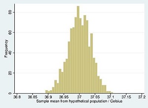
There are a couple of deviations from the ideal bell-shaped curve, but they can be attributed to exceptions and random deviations that always occur in statistical data. Generally speaking, the curve does have a bell shape.

As an opposite example of statistics of a not Normal random variable, consider a distribution of household income in the US. Most likely, the smaller numbers (poor and middle class) will be much more numerous than larger numbers (rich). So, the histogram will be much "heavier" in the smaller numbers, which indicates a not Normal distribution of probabilities.
Here is a histogram for 2010.


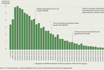
So, just looking at a histogram can convey information about whether the observed random variable is Normally distributed or not.

Counting Frequencies

In many cases we use the properties of Normal distribution of a random variable ξ to evaluate the probabilities of its deviation from its mean value μ:
P{|ξ−μ| ≤ σ} ≅ 0.68
P{|ξ−μ| ≤ 2σ} ≅ 0.95
P{|ξ−μ| ≤ 3σ} ≅ 0.997
where σ is standard deviation of Normally distributed random variable ξ.

This can be used as a test of Normality of statistical distribution based on accumulated sample data.
Having the values our random variable took, we can calculate its sample mean μ and sample standard deviation σ. Then we can calculate the ratio of the number of times values of our random variable fall within σ-boundary around sample meanμ, within 2σ-boundary and within 3σ boundary.
If these ratios are far from, correspondingly, 0.68, 0.95 and0.997, the distribution is unlikely Normal.
Obviously, the more data we have - the better correspondence with the above frequencies we should observe for truly Normal variables.