Unizor is a site where students can learn the high school math (and in the future some other subjects) in a thorough and rigorous way. It allows parents to enroll their children in educational programs and to control the learning process.
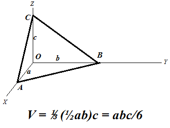
As another example of a double integral as a volume of a solid, consider a pyramid with three plains coinciding with three coordinate planes as follows: base is a right triangle with vertex of the right angle at the origin of coordinates O and catheti OA (along the X-axis) and OB (along the Y-axis); point C on the Z-axis is the top vertex of this pyramid.
Let the lengths of these sides be OA = a OB = b OC = c Our task is to calculate the volume of this pyramid using the double integral and techniques described in the previous lecture.
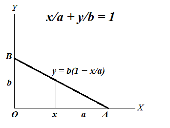
We can consider this problem as the problem of determining a volume of a solid bounded on the top by a plane going through three given points A, B and C and defined on the base triangle ΔOAB lying in the XY-plane.
Since we intend to integrate a function to determine a volume, let's express the plane going through points A, B and C as a function f(x,y) of two arguments x and y - coordinates of a point that belong to a base triangle. Traditional equation of this plane in three-dimensional coordinates is x/a + y/b + z/c = 1 from which follows the functional representation z = f(x, y) = c·(1 − x/a − y/b)
Since our base in not rectangular, we have to pick the primary argument, let it be x changing from 0 to a. The argument y has limits that depend on the value of x in order for point (x, y) to be within our triangle. For each x, therefore, argument y should change from 0 to a point on the hypotenuse of our base triangle. Equation of this line on a plane that goes through points A on the X-axis and B on the Y-axis is x/a + y/b = 1 Therefore, the point on a hypotenuse that corresponds to X-coordinate x is y = b·(1 − x/a)
So, for each primary coordinate x (from 0 to a) coordinate y is changing from 0 to b·(1 − x/a).
Using exactly the same logic as in the previous lecture, we can express the volume of this pyramid as a double integral of function f(x, y) = c·(1 − x/a − y/b) on a base triangle ΔOAB described by primary argument x changing from 0 to a and dependent argument y changing from 0 to b·(1 − x/a).
Now the formula for a volume of our pyramid would be V = ∫0a[∫0b·(1−x/a)f(x,y) dy] dx where f(x, y) = c·(1 − x/a − y/b)
Let's perform the inner integration by y considering x constant. ∫0b·(1−x/a)f(x,y) dy = = ∫0b·(1−x/a)c·(1−x/a−y/b) dy = = c·(1−x/a)∫0b·(1−x/a)dy − (c/b)∫0b·(1−x/a)y dy = = b·c·(1−x/a)²−b·c·(1−x/a)²/2 = = b·c·(1−x/a)²/2 Now, to get the volume of our pyramid, we have to integrate this as a function of x from 0 to a: V =∫0ab·c·(1−x/a)²/2 dx In this case, to integrate it, let's make a substitution t = 1−x/a Then we can express x, its differential dx and limits of integration 0 and a in terms of t: x = a − a·t dx = −a·dt x=0 ⇒ t=1 x=a ⇒ t=0
As a result of this substitution, V =∫10b·c·t²/2 (−a)·dt = = (a·b·c/2)·∫01t²dt = = (a·b·c/2)·(1/3) = a·b·c/6 which corresponds to a known formula for a volume of a pyramid.
Previous lecture introduced a concept of a double integral as a volume of a solid with a rectangular base. In particular, we came to a conclusion that in this case we can integrate, first, by one of the argument and then by another or, equally well, in an opposite order. Rectangular base of a solid allowed such a freedom.
In this lecture we will consider a solid with a circular base and, which is important, the technique of calculating the volume of this solid would be valid for many other types of bases, not necessarily circular. Another important point is that the integration in one order cannot be performed in another order without modifications.
Consider the following problem. Given a smooth function of two variables f(x, y) with non-negative values (that is, f(x, y) ≥ 0), defined on an area bounded by a circle of a radius R with a center at the origin of coordinates, and represented by a surface in (X,Y,Z) coordinate space.
Our task is to find the "volume of a solid" - the measure of a part of coordinate space bounded on the top by a surface representing this function, on the bottom - by X,Y-plane and sides forming a cylindrical surface based on a circle described above, rising on a height determined by the values of our function on the circle's border.
We will follow the same logic as in a case of a rectangular base. The process of approximation starts with dividing our circular base into many small rectangles by lines x=xi (where i∈[0,M], x0=−R, xM=R) and y=yj (where j∈[0,N], y0=−R, yN=R) and constructing rectangular parallelepipeds on the base of these small rectangles with the height equaled to a value of function f(x, y) in the corner of each base rectangle with largest coordinates x and y ("top right corner").
If point (xi, yj) represents the coordinates of a "top right" corner of a small base rectangle and Δxi=xi−xi−1, Δyj=yj−yj−1are sides of this small rectangle, the volume of a constructed rectangular parallelepiped equals to ΔVi,j = f(xi, yj)·Δxi·Δyj
The combined volume of all these parallelepipeds approximates the volume of our solid. With increasing number of small base rectangles and, correspondingly, decreasing their dimensions we assume that there is a limit of the combined volume of all these parallelepipeds. It can be proven that under certain conditions of smoothness of our function f(x, y) the limit does exist and is unique, regardless of the way how exactly we divide the domain of our function into small rectangles, as long as their dimensions are converging to zero (or, more precisely, the dimensions of the largest among them converges to zero).
Now let's consider how we can summarize the volumes of all parallelepipeds constructed on the basis of small rectangles. We cannot summarize all xi and yj, as we did in a case of a rectangular base, because many of them will go outside of a circle where the function is undefined. Instead, let's use the following logic. We will choose one of the arguments, let's say x, as the "primary" and will change it from x0=−R to xM=R, that is through all values of xi. For each chosen x=xi we will choose only those values of y that fall within a circle of radius R, that is from −√R²−x² to √R²−x².
Therefore, while the limits of summation by "primary" argument x are all its values from x0=−R to xM=R, the limits of summation by "secondary" argument y depend on the value of "primary" x as specified above. This dependence of the limits of summation (and, subsequently, integration) by secondary argument on the value of the primary one is the only difference of this case of circular base from the previously considered rectangular base.
Decreasing the intervals between division points by both arguments and going to a limit, we will have, firstly, an integral by a primary argument x in limits from −R to R and, for each value of x we will have to integrate by a secondary argument y in limits that depend on the value of primary argument x - from −√R²−x² to √R²−x².
The final formula would look like this: ∫−RR[∫−√R²−x²√R²−x²f(x, y) dy] dx
Let's use this formula for calculating the volume of a cylinder with f(x, y)=H - the height of a cylinder. According to the rules of geometry, the volume of a cylinder equals to a product of an area of a base by its height, so we have to get the answer V=πR²H. Let's check if we get it through integration.
∫−RR[∫−√R²−x²√R²−x²H dy] dx = ∫−RR[2H√R²−x²] dx Substitute x=R·sin(t), where −π/2 ≤ t ≤ π/2 Then √R²−x² = R·cos(t), dx=R·cos(t) dt, getting ∫−π/2π/2[2HRcos(t)]R·cos(t)dt = 2HR²∫−π/2π/2cos²(t)dt
To simplify it further, use the trigonometric identity cos(2t) = cos²(t)−sin²(t) = = 2cos²(t) −1 from which we derive cos²(t) = [cos(2t)+1]/2 Our integral now looks like this 2HR²∫−π/2π/2[cos(2t)+1]/2 dt = = HR²∫−π/2π/2[cos(2t)+1]dt = = HR²∫−π/2π/2cos(2t) dt + HR²∫−π/2π/2dt Indefinite integral (anti-derivative) of cos(2t) is (1/2)·sin(2t). Therefore, the first integral in this sum equals to ∫−π/2π/2cos(2t) dt = (1/2)·[sin(2π/2)−sin(−2π/2)] = (1/2)·[sin(π)−sin(−π)] = 0
The second integral in a sum above equals to ∫−π/2π/2dt = π/2 − (−π/2) = π Therefore, the result of integration is HR²·π = πR²H which corresponds to results from geometry.
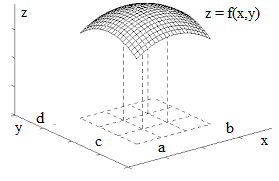
Consider the following problem. Given a smooth function of two variables f(x, y) (we will always consider smooth functions in terms of continuity and sufficient differentiability), with non-negative values (that is, f(x, y) ≥ 0), defined on a closed rectangle a ≤ x ≤ b, c ≤ y ≤ d and represented by a surface in (X,Y,Z) coordinate space.
In the following we will use the word "area" in a sense of a two-dimensional part of a plane and as a quantitative measure of this part of plane. The context would clarify which one it is used in every case.
Our task is to find the "volume of a solid" - the measure of a part of coordinate space bounded on the top by a surface representing this function, on the bottom - the X,Y-plane and on the four sides by planes x = a, x = b, y = c and y = d.
There is no ready to use formula for such a volume. We do know how the volume of a rectangular parallelepiped is defined, it is a product of its three dimensions - length multiplied by width, multiplied by height, but not of such a complicated figure as the one we consider now.
We really have to define what the volume of this figure is and then attempt to calculate it based on values of function f(x, y) on a rectangle [a, b, c, d]. We did have a similar problem in Geometry with the volume of solids and approached it as a sequence of approximations of a complex figure with simple ones. Let's do the same now.
We will use certain intuitive considerations to define the volume of a solid and will prove that this definition is mathematically valid.
The process of approximation starts with dividing rectangle [a, b, c, d] into many small rectangles by lines x=xi (where i∈[0,M], x0=a, xM=b) and y=yj(where j∈[0,N], y0=c, yN=d) and constructing M·N rectangular parallelepipeds on the base of these small rectangles with the height equaled to a value of function f(x, y) in the corner of each base rectangle with largest coordinates x and y ("top right corner").
If point (xi, yj) represents the coordinates of a "top right" corner of a small base rectangle and Δxi=xi−xi−1, Δyj=yj−yj−1are sides of this small rectangle, the volume of a constructed rectangular parallelepiped equals to ΔVi,j = f(xi, yj)·Δxi·Δyj
The combined volume of all these parallelepipeds approximates the volume of our solid. With increasing number of small base rectangles and, correspondingly, decreasing their dimensions we assume that there is a limit of the combined volume of all these parallelepipeds. It can be proven that under certain conditions of smoothness of our function f(x, y) the limit does exist and is unique, regardless of the way how exactly we divide the domain of our function into small rectangles, as long as their dimensions are converging to zero (or, more precisely, the =dimensions of the largest among them converges to zero).
Now let's consider how we can summarize the volumes of all parallelepipeds constructed on the basis of small rectangles. There are two simple methods.
1. We can go from one point y=yj to another, varying index j from 1 to N and for each value of y=yj summarize the volumes of all parallelepipeds based on all values of x=xi, varying index i from 1 to M. So, for each index j we calculate the sum of all Vi,j, varying index i. Then we summarize these sums by index j deriving with an approximate volume VM·N = Σj∈[1,N]Σi∈[1,M] Vi,j = = ΣjΣi f(xi, yj)·Δxi·Δyj = = Σj[Σi f(xi, yj)·Δxi]·Δyj
2. On the other hand, we can go from one point x=xi to another, varying index i from 1 to M and for each value of x=xisummarize the volumes of all parallelepipeds based on all values of y=yj, varying index j from 1 to N. So, for each index i we calculate the sum of all Vi,j, varying index j. Then we summarize these sums by index i deriving with an approximate volume VM·N = Σi∈[1,M]Σj∈[1,N] Vi,j = = ΣiΣj f(xi, yj)·Δxi·Δyj = = Σi[Σj f(xi, yj)·Δyj]·Δxi
Both approaches to summarizing the volumes of small parallelepipeds should result in the same value of a combined volume.
Let's examine now what happens with both our formulas for total volume when the rectangles are getting smaller and smaller.
Recall the definition of a definite integral of function φ(t) on a segment p ≤ t ≤ q as a limit of sums of areas of rectangles obtained by dividing segment [p,q] into small pieces: Σk φ(tk)·Δtk→ ∫pqφ(t) dt
We can now say that Σj f(xi, yj)·Δyj converges to φ(xi) = lim Σj f(xi, yj)·Δyj = = ∫cdf(xi, y) dy under condition of maximum among Δyj converges to zero. Then we continue with the second summation getting Σi[Σj f(xi, yj)·Δyj]·Δxi → → Σi[∫cdf(xi, y) dy]·Δxi → → ∫ab[∫cdf(xi, y) dy] dx
On the other hand, we can similarly state that Σi f(xi, yj)·Δxi converges to ψ(yj) = lim Σi f(xi, yj)·Δxi = = ∫abf(x, yj) dx under condition of maximum among Δxi converges to zero. Then we continue with the second summation getting Σj[Σi f(xi, yj)·Δxi]·Δyj → → Σj[∫abf(x, yj) dx]·Δyj → → ∫cd[∫abf(x, y) dx] dy
But these are supposed to be the same results since the difference is only in the order of summation. The sums are the same, therefore the limits are the same, therefore we can write this limit as a double integral: ∫cd∫abf(x, y) dx dy or ∫ab∫cdf(x, y) dy dx
Both are the same and constitute two integrations of function f(x, y) performed consecutively, either by x from a to b (keeping y as a constant) and then by y from c to d or, in reverse, first by y from c to d (keeping x as a constant) and then by x from a to b.
Partial Differential Equations Solution to Heat Equation
Our purpose is to solve the heat equation that describes the dynamics of temperature distribution within a thin rod and looks like this: ∂T(t,x)/∂t = a²·∂²T(t,x)/∂x² where t - time, x - distance of a point on a thin rod from its edge, T(t,x) - temperature at time t of a point on a rod at distance x from its edge, a - constant that depends on physical characteristics of a rod.
This is a partial differential equation for function T(t,x) describing the distribution of temperature T within a thin rod at time t at location with X-coordinate x, assuming it's positioned along the X-axis with the left edge at x=0.
First of all, let's state that this distribution of temperature depends not only on the equation itself, which reflects dynamics of heat movement within a rod, but also depends on the initial conditions - what was the temperature at different locations of a rod at time t=0, described by function T(x,0).
Another type of condition that might be necessary to take into account is so-called boundary condition. It plays an important role in cases when edges of a rod are maintained at certain (not necessarily fixed) temperature all the time, which can be described by functions T(0,t) and T(L,t) (here L is the length of a rod).
Now we are ready to solve the equation. Let's find a solution to our partial differential equation in a form T(t,x) = f(t)·g(x) We don't know if we will succeed on this way, but it's worth to try, since this relatively simple approach might bring us to solution. If it does, great. If it does not, at least, we tried.
Then ∂T(t,x)/∂t = f'(t)·g(x) ∂²T(t,x)/∂x² = f(t)·g''(x) Now our heat equation looks like f'(t)·g(x) = a²·f(t)·g''(x) or f'(t)/f(t) = a²·g''(x)/g(x) Now we have a peculiar situation, when a function of t is equal to a function of x. The only possibility of this might be if both functions are constants that are equal to each other. Therefore, f'(t)/f(t) = A and a²·g''(x)/g(x) = A where A - some unknown constant that might be determined using initial conditions.
These are two ordinary differential equations, both types were addressed in the previous lectures. Let's get to their solutions.
The equation for f(t) is solved as follows: df/f = A·dt Integrating both sides results in ln|f| = A·t + C (where C - any constant) |f(t)| = eA·t+C or, considering C is any constant, f(t) = C·eA·t
It's easy to check that this is a solution since f'(t) = C·A·eA·t and f'(t)/f(t) = A
The equation for g(x) is a linear equation of the second order, considered in a prior lecture about oscillation of a spring. We can represent it as g''(x) − (A/a²)·g(x) = 0 We will look for its solution in a form g(x) = eλ·x where λ - any complex number. Since g''(x) = λ²·eλ·x we come to a simple quadratic equation for λ: λ² − A/a² = 0 with solutions λ = ±(1/a)·√A This results in solutions for g(x): g(x) = C1·e(1/a)·√A·x + C2·e−(1/a)·√A·x
General solution to a heat equation can now be represented as T(t,x) = f(t)·g(x) = = C·eA·t·(C1·e(1/a)·√A·x + C2·e−(1/a)·√A·x) where C, C1 and C2 are unknown constants, that can be defined only if additional conditions (initial conditions or boundary conditions) are given.
What remains is analysis of our solution for a purpose to get only real component of it, ignoring imaginary part, and apply initial condition on distribution of temperatures at time t=0, like T(0,x)=u(x), and boundary conditions (if applicable) T(t,0)=T0 and T(t,L)=TL in order to determine unknown constants. These are purely technical issues and lie outside the scope of this course.
Since we talked about ordinary differential equations, where a function of one argument together with its derivatives participates in the equation, we might as well touch on differential equations, where function of two (or more) arguments together with its partial derivatives participates in the equation. These equations are called partial differential equations.
In order to present this material in a more practical light and to emphasize the importance of differential equations (particularly, partial) in practical applications, let's discuss one particular physical process that naturally leads to partial differential equations.
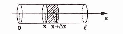
Let's imagine an insulated thin metal rod heated on one end and examine how its temperature T at different distance from the edge changes with time. We assume that the rod is stretched along the X-axis with its heated end at origin. The distance from this end to any point on a rod is X-coordinate of this point. Time t will be measured from the moment the heat is applied to the edge at x=0.
Considering our rod is insulated and thin, we can safely assume that the heat dissipates only along its length from point x=0 towards the other edge, and the rod's temperature is a function of two arguments: distance x from the edge and time t: T = T(t,x) The illustration below will be handy in our analysis.
Before embarking on calculations let us remind a few physical properties that affect the process of heat dissipation.
1. Heat Q - a form of energy manifested in vibration of molecules of an object. It is measured in the same units as energy.
2. Temperature T - a measure of intensity of the molecular vibration. It is measured in degrees of different scales.
3. Specific heat capacity C - an amount of energy (heat) needed to increase temperature of a unit of mass by a unit of temperature. It is assumed to be a constant for any specific material within reasonable range of temperatures and precision. If an object of mass m increased in temperature by ΔT, it consumed ΔQ=C·m·ΔT units of heat (energy).
4. Thermal conductivity k - a measure of how fast molecular vibration is transferred within an object. It was experimentally established that the amount of heat transferred from one zone of an object to another per unit of time through a unit of area on the boundary between these zones is proportional to a rate of change of temperature at this boundary and depends on the qualities of the material. For every material it is a constant within a reasonable range of temperatures. In one-dimensional case on an above picture of a thin rod that has area S of crosscut, when the heat is transformed through a point x and the rate of change of temperature at that point and at that time is ∂T(t,x)/∂x, the amount of heat that goes through during time Δt can be calculated as ΔQ = −k·S·Δt·∂T(t,x)/∂x Minus in this equality reflects that heat is transferred from hot to cold area and, therefore, the partial derivative of temperature T by x is negative, while energy must be positive.
Now we are ready to connect all the parameters mentioned above into one heat equation.
Consider a part of a thin rod from point x to point x+Δx. As the heat dissipates from left to right, during the time Δt certain amount of heat enters this area through crossing at point x and certain amount of heat exits this area through crossing at point x+Δx.
The heat entering through crossing at point x measures ΔQin = −k·S·Δt·∂T(t,x)/∂x The heat exiting through crossing at point x+Δx measures ΔQout = −k·S·Δt·∂T(t,x+Δx)/∂x
The difference between them is an amount of heat that contributed to a rise in temperature of the part of a rod from x to x+Δx. This difference equals to (A) ΔQ+ = k·S·Δt·[∂T(t,x+Δx)/∂x − ∂T(t,x)/∂x]
On the other hand, the heat ΔQ+, consumed by a part of a rod of length Δx, area of crosscut S and specific heat capacity C should increase the temperature by ΔT related to this heat as ΔQ+ = C·m·ΔT where m is a mass of this part of a rod, that can be calculated as m = ρ·S·Δx where ρ is a mass of a unit of volume of the material this rod is made of. Therefore, (B) ΔQ+ = C·ρ·S·Δx·ΔT
From equations (A) and (B) we derive the following equality: C·ρ·S·Δx·ΔT = k·S·Δt·[∂T(t,x+Δx)/∂x − ∂T(t,x)/∂x] This can be transformed into ΔT/Δt = [k/(C·ρ)]·[∂T(t,x+Δx)/∂x−∂T(t,x)/∂x]/Δx
When Δt→0 and Δx→0 our equation can be represented as ∂T(t,x)/∂t = [k/(C·ρ)]·∂²T(t,x)/∂x²
Traditionally, this heat equation is written as ∂T(t,x)/∂t = a²·∂²T(t,x)/∂x² where a² = k/(C·ρ)
Higher Order Ordinary Differential Equations - Hooke'sLaw
Our next subject is Hooke's Law. This law describes the force of a stretched or compressed spring.
Let's assume that we have a weightless spring horizontally lying on the frictionless table along an imaginary X-axis and fixed at the left end. Its free right end is at coordinate x=0 and there is a point mass m attached to this free end of a spring. Then we stretch this spring by pulling the right end from a neutral position by certain length x.
Obviously, the spring exerts a force to compress back to a neutral position. The Hooke's Law states that within certain reasonable boundaries (no over-stretching) this force is proportional to a difference in length between a stretched string and a string in a neutral position. This is expressed by the formula F = −k·x where F is the force exerted by a spring, x is a displacement of the free end of a spring from a neutral position, k is a positive constant that characterizes a spring (called a spring constant) and the minus sign signifies that the direction of force is opposite to the direction of displacement because, if displacement is positive (stretching), the force is directed towards negative direction of the X-axis and, if displacement is negative (compression), the force is directed towards positive direction of the X-axis.
Now recall Newton's Second Law that related the force and acceleration F = m·a where F is the force, m is the mass of an object and a is its acceleration.
From these two laws we conclude that m·a = −k·x
Since x is a distance along the X-axis and a is an acceleration along this axis, that is a second derivative from a distance by time, we came up with the following differential equation m·x''(t) = −k·x or m·x''(t) + k·x(t) = 0 or x''(t) + (k/m)·x(t) = 0 This is a second order ordinary differential equation. It is a little more complex than we considered in a lecture about acceleration and Newton's Second Law. Let's try to solve it.
First of all, let us mention that even a simple guessing in this and many other cases is a good choice. Recall that first derivative of sin() is cos() and the first derivative of cos(), that is the same as the second derivative of sin(), is −sin(). So, the equation x''(t)+x(t)=0 has a solution x=sin(t). This is very close to what we have. Adding a factor α to an argument might help to satisfy multipliers in our equation: if x(t)=sin(α·t) then x'(t)=α·cos(α·t) and x''(t) = −α²·sin(α·t) and, therefore, x''(t)+α²·x(t) = 0 Now we can choose α to satisfy α²=k/m, and the solution to our equation is found.
Guessing is good, when we can guess (as in this case), but guessing might not be successful and, even if you managed to guess one solution, it's not a guarantee that all solutions are found. By the way, if we start with cos(), we will also find a solution. So, let's have some theory.
Our differential equation belongs to a class of linear ordinary differential equations of second order with constant coefficients and can be generalized as x''(t) + p·x'(t) + q·x(t) = 0
As we saw above, functions sin() and cos() might be involved in a solution. Analogous quality of derivative being similar to a function itself is possessed by exponential functions. Recall also that exponential functions with complex exponent is related to trigonometric function through famous Euler's formula eit = cos(t) + i·sin(t) So, exponential functions, in some way, are more general than trigonometric, they encompass them. Therefore, it's only natural to look for a solution in terms of exponential functions. Let's try.
Assume, we are looking for a solution to our equation in the form x(t)=eλ·t, where λ might be any (including complex to accommodate trigonometric functions) number. Then derivatives of this function are: x'(t) = λ·eλ·t x''(t) = λ²·eλ·t Putting this into our equations, we get λ²·eλ·t + λ·p·eλ·t + q·eλ·t = 0 Canceling eλ·t, we get a simple quadratic equation for λ called a characteristic polynomial of a given differential equation: λ² + p·λ + q = 0 Since this equation always has two solutions λ1 and λ2 among complex numbers, we will have two particular solutions to our differential equation: eλ1·t and eλ2·t Finally, any linear combination of these two particular solutions will also be a solution (since our differential equation is linear and a derivative of linear combination of functions is a linear combination of derivatives). Therefore, we can state the general solution to our differential equation: x(t) = C1·eλ1·t+C2·eλ2·t which depends on two unknown complex constants C1and C2, their values can be defined only if some initial conditions of the movement are given.
Let's get back to a movement of a spring. Our initial equation x''(t) + (k/m)·x(t) = 0 has a characteristic polynomial λ² + k/m = 0 (where both k and m are positive) with two solutions: λ1 = √(k/m)·i and λ2 = −√(k/m)·i where i²=−1 is an imaginary unit in the field of complex numbers.
Let ω = √(k/m). Now we can represent the general solution to a movement of a spring based on the Hooke's Law as follows: x(t) = C1·eiωt + C2·e−iωt This expression can be easily transformed using Euler's formula into x(t) = C1·cos(ωt)+i·C1·sin(ωt)+ +C2·cos(−ωt)+i·C2·sin(−ωt)
Since C1 can be represented as A1+i·B1 and C2 can be represented as A2+i·B2, where A1, B1, A2 and B2 are undefined unknown real numbers, the whole expression can be represented as D1·cos(ωt) + D2·sin(ωt) + i·Z where coefficients D1 and D2are any real numbers and i·Z represents purely imaginary part.
Since we deal with physics, we should exclude all imaginary solutions and leave only those, where D1 and D2 are real numbers. So, the general physical solution looks like x(t) = D1·cos(ωt) + D2·sin(ωt) where D1 and D2 are undefined unknown real numbers.
In our experiment we have stretched a string by some known distance from a neutral position and let it spring back. That means, we know the initial position x(0)=d and initial speed x'(0)=0. These initial conditions are sufficient to determine two unknown constants in our equation of a motion: x(0)=d ⇒ ⇒ D1cos(0)+D2sin(0)=d ⇒ D1 = d x'(0)=0 ⇒ ⇒ −ω·D1sin(0)+ω·D2cos(0)=0 ⇒ D2 = 0
The final form of an equation of motion is x(t) = d·cos(ωt) where ω = √(k/m), k is a spring constant, m is a point mass at its free end and d is the initial distance we have stretched a spring from its neutral position. As seen from this equation of motion, a free end of a spring with a mass attached to it will indefinitely oscillate around the neutral point. The end.
Higher Order Ordinary Differential Equations - Acceleration
Differential equations can include derivatives of higher order - second derivative, third, etc. Probably, most common equations of this type are those with the second order derivative. These equations are very often occur in science, especially in Physics. Let's address these equations and approaches to solve them.
Our first subject is a concept of acceleration and Newton's Second Law.
Recall that speed measures how fast a distance from some starting point changes, that is, if this distance is represented as a function x(t) of time t, speedv(t) at any moment t is the first derivative of distance by time: v(t) = x'(t) = dx/dt
But speed does not have to be constant, we can move faster, increasing our speed (accelerating), or slower, decreasing it (decelerating). To measure how fast our speed changes with time, as usually, when we want to measure how fast anything changes with time, we use a derivative. Differentiating speed (a function of time) by time we obtain this measure of change of speed at any moment. This derivative of speed by time is called accelerationa(t): a(t) = v'(t) = dv/dt = = x''(t) = d²x/dx² That is, acceleration is the second derivative of distance by time.
Newton's Second Law states that the forceF applied to an object and the accelerationa this object obtains as a result of this application of force are related as follows: F = m·a where m is the object's mass (presumed constant).
Assuming that our motion occurs along a straight line with coordinates and, therefore, the position of an object is defined by its X-coordinate x(t), Newton's Second Law is an ordinary differential equation of second order because acceleration is the second derivative of the X-coordinate of an object: F(t) = m·x''(t) Usually our task is to find where exactly our object is located (that is, its X-coordinate), if the force, as a function of time, is given.
Consider a case when there is no force applied to an object, that is F(t)=0. Then, according to the Newton's Second Law, 0 = m·a(t) from which we derive a(t)=0 Since a(t)=v'(t), we can find the speed: v'(t)=0 ⇒ v(t) = C (where C is an unknown constant) ⇒ x'(t) = C ⇒ x(t) = C·t + D (where D is another unknown constant)
That concludes the solution of our differential equation of the second order, and the solution includes two unknown constants that cannot be determined from the equation alone. It's understandable since we don't know initial position of an object on the coordinate axis x(0) and the initial speed it moved v(0). These two additional pieces of information (initial conditions) are needed to determine unknown constants participating in the solution. If x(0)=x0 and v(0)=v0, we can easily determine x0 = D and v0 = C which results in the final equation of motion of an object, to which no forces are applied (or, more generally, all forces applied to it are balancing each other). x(t) = x0 + v0·t
By solving the above differential equation of the second order, we have mathematically derived the Newton's First Law as a consequence of the Second Law. Newton's First Law (law of inertia) states that if the sum of all forces applied to an object is zero, then the object at rest will continue to stay at rest (its speed is and will be 0) and objects moving at some speed will continue to move with the same speed and direction (its speed is constant).
Now consider a case when the force applied to an object is not zero, but constant, that is F(t)=P (const). Let's attempt to solve our differential equation in this case to determine the coordinate of an object as a function of time x(t). F(t)=P=m·a(t)=m·v'(t) where P is a known constant. This implies that acceleration a(t) must be a known constant and equals to P/m. Let's use symbol a instead of a(t) to signify this. Since a=v'(t), we derive v(t) = a·t + C where C is an unknown constant. Then x'(t) = a·t + C ⇒ x(t) = a·t²/2 + C·t + D where D is another unknown constant. To determine two unknown constants we need additional information - initial conditions. Assume that the original position of an object is x(0)=x0. This allows to determine D=x0. If initial speed v(0)=v0 is known, we can determine C=v0. So, the final equation of the motion, when a constant force is applied is x(t) = a·t²/2 + v0·t + x0
In general, if the force is variable and/or the mass is variable, from Newton's Second Law we can construct a differential equation of the second order, where the second derivative is explicitly represented by a known function: F(t) = m(t)·x''(t) ⇒ x''(t) = F(t)/m(t) ⇒ d/dt[x'(t)] = F(t)/m(t) ⇒ x'(t) = ∫[F(t)/m(t)]dt ⇒ x(t) = ∫{∫[F(t)/m(t)]dt}dt
As we see, Newton's Second Law presents the simplest kind of ordinary differential equation of the second order. It can be solved by double integration. It should not be forgotten that in the process of each integration there will appear an unknown constant, to get its value an initial condition should be known and applied.
Standard form of linear ordinary differential equations is f(x)·y' + g(x)·y + h(x) = 0 As the first step, we can divide all members of this equation by f(x) (assuming it's not identically equal to 0), getting a simpler equation y'+u(x)·y+v(x) = 0 The suggested solution lies in the substitution y(x)=p(x)·q(x), where p(x) and q(x) are unknown (for now) functions. Express y'(x) in terms of p(x) and q(x): y' = p·q'+q·p' Substitute this into our equation: p·q'+q·p'+u·p·q+v = 0 Let's simplify this p(q'+u·q)+q·p'+v = 0 If there are such functions p(x) and q(x) that satisfy conditions (1) q'+u·q = 0 and (2) q·p'+v = 0 our job would be finished. Let's try to find such functions. From the equation (1) in our pair of equations we derive q'/q = −u, which can be converted into dq(x)/q(x) = −u(x)·dx that can be solved by integrating: ln(q(x)) = −∫u(x)·dx q(x) = e−∫u(x)·dx Once q(x) is found, we solve the equation (2) for p(x): p'(x) = −v(x)/q(x), which can be integrated to find p(x) = −∫v(x)/q(x) dx and, consequently, y(x)=p(x)·q(x) can be fully determined. Let's consider a few examples.
Example 1
Solve the following linear differential equation y' + y + x = 0
Let's look for a solution in a form y(x)=p(x)·q(x) Then y'(x) = p'(x)·q(x)+p(x)·q'(x) Our equation looks like this now p'·q+p·q' + p·q + x = 0 Factor out p, getting p·(q'+q) + (p'·q+x) = 0 We will try to find p(x) and q(x) to separately bring to zero q'+q and p'·q+x. Let's look for a function q(x) that brings expression q'+q to zero: q'+q = 0 dq/q = −dx ∫dq/q = −∫dx ln(q) = −x + A (where A is any constant) q(x) = B·e−x (where B=eA, so it represents any positive number) Next, let's find a solution to p'·q+x = 0 p'·B·e−x+x = 0 p(x) = −(1/B)·∫x·exdx This integral can be found using the "by parts" technique: p(x) = −(1/B)·(x·ex−∫exdx) = = −(1/B)·(x·ex−ex−C) = = −(1/B)·(x−1)·ex+C/B (where B is any positive constant and C is any constants) Now let's find y(x)=p(x)·q(x): y(x) = [−(1/B)·(x−1)·ex+C/B]·[B·e−x] = = 1−x+C·e-x
Solve the following linear differential equation y'·cos(x) + y·sin(x) − 1 = 0
First of all, let's normalize it by dividing by cos(x), noticing that sin(x)/cos(x)=tan(x) and 1/cos(x)=sec(x): y' + y·tan(x) − sec(x) = 0 Let's look for a solution to this equation in a form y(x)=p(x)·q(x) Then y'(x) = p'(x)·q(x)+p(x)·q'(x) Our equation looks like this now: p'·q+p·q'+p·q·tan(x)−sec(x) = 0 Factor out p, getting p·(q'+q·tan(x))+p'·q−sec(x) = 0 First, let's find function q(x) such that q' + q·tan(x) = 0 It can be solved using the technique of separation: dq/q = −tan(x)dx Since [ln(x)]' = 1/x and [cos(x)]' = −sin(x), the last equation can be transformed into d(ln(q)) = d(cos(x))/cos(x) d(ln(q)) = d(ln(cos(x))) Now it's easy to integrate, the result is ln(q) = ln(cos(x))+C where C - any real number, from which, raising number e to both left and right sides, follows that q = D·cos(x) (new constant D=eC represents any positive number) Now let's find function p(x) such that p'·q − sec(x) = 0 Substitute already found q(x) getting p'·D·cos(x) − sec(x) = 0 p'(x) = (1/D)·(1/cos²(x)) p(x) = (1/D)·∫dx/cos²(x) = = (1/D)·[tan(x) + E] where D and E are constants (D - any positive, E - any real) Let's determine y=p·q now. y(x) = p(x)·q(x) = = (1/D)·[tan(x) + E]·D·cos(x) = = sin(x) + E·cos(x)
Let's check this result. y'(x) = cos(x)−E·sin(x) y'·cos(x) + y·sin(x) − 1 = = cos²(x)−E·sin(x)·cos(x) + sin²(x)+E·cos(x)·sin(x)−1 = = sin²(x) + cos²(x) −1 = 0 which proves the correctness of our answer.
Example 3
Solve the following differential equation ln(x·y'+y) = ln(2x)+x²
It's not linear, but can be made linear if we raise e to a power defined by its left and right sides, getting x·y'+y = 2x·ex² Let's normalize it by dividing by x: y' + y/x = 2ex² Now it's a linear equation that we know how to solve. Let's look for a solution in a form y(x)=p(x)·q(x) Then y'(x) = p'(x)·q(x)+p(x)·q'(x) Our equation looks like this now p'·q+p·q' + p·q/x = 2ex² Factor out p, getting p·(q'+q/x) + p'·q = 2ex² We will try to find p(x) and q(x) to separately (a) bring to zero q'+q/x and (b) equalize p'·q with 2ex². Let's solve equation (a) and look for a function q(x) that brings expression q'+q/x to zero: q'+q/x = 0 dq/q = −dx/x ∫dq/q = −∫dx/x ln(|q|) = −ln(|x|) + A where A - any constant. Raising e to both sides of this equation, we get |q| = B/|x| where B=eA - any positive number. Let's get rid of absolute values in the above equation by allowing B to be any non-zero real number, so q = B/x Substitute it to equation (b): p'·B/x = 2ex² p(x) = (1/B)∫2x·ex²·dx Since derivative of x² is 2x, p(x) = (1/B)∫ex²·d(x²) Now we can integrate directly: p(x) = (1/B)ex² + C where C is any real number. This allows to express the solution to our differential equation in the form y(x) = p(x)·q(x) where p(x) = (1/B)ex² + C and q(x) = B/x That produces y = ex²/x + C/x = (ex²+C)/x where C - any real number.
Checking: y' = −(ex²+C)/x² + ex²·2x/x = = ex²·(2−1/x²) −C/x² y/x = ex²/x² + C/x² y' + y/x = 2ex², which corresponds to the original equation after multiplying both sides by x and taking logarithm. The end.
We have defined homogeneous ordinary differential equations of the first order as an equation F(x, y, y')=0 which does not change if we replace x with λ·x and y with λ·y, where λ - any real number not equal to zero. In other words, F(x, y, y') = F(λ·x, λ·y, y') Examples: F(x, y, y') = y'+y/x F(x, y, y') = 3y'+x·y/(x²+y²) etc.
The recommended technique to solve these equations is to substitute function y(x) with x·z(x) and solve the equation for z(x), after which determine y(x)=x·z(x).
Let's solve a few equations of this kind.
Example 1
Check for homogeneousness and solve the following equation: x·y' = x·sin(y/x) + y
Checking for homogeneousness. Substitute x with λ·x and y with λ·y: λ·x·y' = λ·x·sin(λ·y/(λ·x)) + λ·y Obviously, λ cancels out completely, which proves homogeneous character of the equation. Now let's solve this equation using the substitution z(x)=y(x)/x, which results in y(x)=z(x)·x, and express the initial equation in terms of x, z and z'. x·(z'·x + z) = x·sin(z) + z·x Simplifying: z'·x + z = sin(z) + z z'·x = sin(z) dz/sin(z) = dx/x ∫dz/sin(z) = ∫dx/x The right side is easy, the integral equals to ln(|x|)+C. The left side is more involved. ∫dz/sin(z) = = ∫dz/(2sin(z/2)·cos(z/2)) = = ∫d(z/2)/(sin(z/2)·cos(z/2)) Substitute u=z/2, getting ∫du/(sin(u)·cos(u)) = = ∫cos(u)d(u)/(sin(u)·cos²(u)) = = ∫d(sin(u))/(sin(u)·cos²(u)) Substitute t=sin(u), getting ∫dt/[t·(1−t²)] The polynomial in the denominator is t·(1−t²) = t·(1−t)·(1+t) Its inverse can be represented as 1/t − 1/[2(1+t)] + 1/[2(1−t)] which makes our integral equal to ∫{[2/t−1/(1+t)+1/(1−t)]/2}dt The last expression can be represented as a sum of three integrals, the result of integration is: ln(|t|) − ln(|1+t|)/2 − ln(|1−t|)/2 where t=sin(z/2) This leads us to a final solution of our differential equation. ln(|sin(z/2)|) − ln(1+sin(z/2))/2 − ln(1−sin(z/2))/2 = ln(|x|)+C and then we should substitute z=y/x to get the final expression ln(|sin(y/2x)|) − ln(1+sin(y/2x))/2 − ln(1−sin(y/2x))/2 = ln(|x|)+C Using this as an exponent, we come up with an expression without logarithms |sin(y/2x)| /[(1+sin(y/2x))·(1−sin(y/2x))] = C·|x| A simplification in the denominator results in |sin(y/2x)| / cos²(y/2x) = C·|x| We leave it "as is" without resolving for y(x).
Example 2
Check for homogeneousness and solve the following equation: [(y − x·y')/x]x = ey
Checking for homogeneousness. Substitute x with λ·x and y with λ·y: [(λy − λx·y')/λx]λx = eλy Cancel λ in the ratio, getting: [(y − x·y')/x]λx = eλy This can be written as {[(y − x·y')/x]x}λ = [ey]λ Raising both sides to power 1/λ (or, which is the same, extracting a root of power λ) we come to the original equation, which proves homogeneous character of the equation. Now we will solve it using the recommended technique. Substitute z(x)=y(x)/x, which results in y(x)=z(x)·x and express the initial equation in terms of x, z and z'. The expression for a derivative y' is: y' = (z·x)' = z'·x+z New equation is, therefore, [(z·x − x·(z'·x+z))/x]x = ez·x Simplifying it by raising to power 1/x both sides (or, equivalently, extracting a root of power x): [(z·x − x·(z'·x+z))/x] = ez Cancel x: z − (z'·x+z) = ez Cancel z: −z'·x = ez This equation is separable, let's separate x from x, getting −e−z·dz = dx/x Ready to integrate: ∫−e−z·dz = ∫dx/x e-z = ln(x)+C (assuming for simplicity positive only sign for x, so integral on the right is ln(x) instead of ln(|x|)) From the last equation we derive: −z = ln(ln(x)) + C z = −ln(ln(x)) + C Now we can use it to find an expression for y: y = −x·ln(ln(x)) + C
Solution must be checked. It's easier, instead of checking the original equation [(y − x·y')/x]x = ey to check the equality of logarithms from both sides: x·ln[(y − x·y')/x] = y or, simpler, ln(y/x − y') = y/x where we should substitute y = −x·ln(ln(x)) + C and y' = −ln(ln(x))−x·(1/ln(x))·(1/x) or, simpler, y' = −ln(ln(x)) − 1/ln(x) Let's disregard constant C in this checking to make manipulations simpler. Then, since y/x = −ln(ln(x)) we will have to check that ln(−ln(ln(x)) + ln(ln(x)) + 1/ln(x)) = −ln(ln(x)) Canceling opposite positive and negative members under logarithm on the left, we come to an obvious equality ln(1/ln(x)) = −ln(ln(x)) which proves the correctness of our solution.
Example 3
Check for homogeneousness and solve the following equation: x·y·y' = (x+y)²
Checking for homogeneousness. Substitute x with λ·x and y with λ·y: λx·λy·y' = (λx+λy)² λ²x·y·y' = λ²(x+y)² Obviously, λ cancels out, and we get the same original equation. Now let's solve it by substituting z(x)=y(x)/x, which results in y(x)=z(x)·x and express the initial equation in terms of x, z and z'. The expression for a derivative y' is: y' = (z·x)' = z'·x+z So, our equation looks like x·(z·x)·(z'·x+z) = (x+z·x)² Simplifying by opening all parenthesis, we get x²·(x·z·z'+z²) = x²·(1+z)² x·z·z'+z² = (1+z)² x·z·z' = 1+2z This equation can be solved using the method of separation. z·dz/(1+2z) = dx/x Integrating the left side of this equation: ∫z·dz/(1+2z) = = (1/2)∫(1+2z−1)·dz/(1+2z) = = (1/2)[∫dz − ∫dz/(1+2z)] = = (1/2)[z−(1/2)ln(1+2z)] + C Integrating the right side of the equation: ∫dx/x = ln(x) + C Since integral of both sides are equal, (1/2)[z−(1/2)ln(1+2z)] = = ln(x)+ C which can be simplified 2z − ln(1+2z) = 4ln(x) + C Though this equation for z(x) cannot be easily solve for z, it allows to replace the original differential equation for y with purely algebraic one, replacing z with y/x: (A) 2y/x − ln(1+2y/x) = = 4ln(x) + C This is the final algebraic answer to our differential equation. Though it's not resolved for y(x), it's still the best solution we can come up with.
Solution must be checked. If this equality that includes function y(x) is correct, derivatives of both parts are also equal. Let's differentiate them both. −2y/x² + 2y'/x − (1/(1+2y/x))·(−2y/x²+2y'/x) = 4/x Simplifying by multiplying by x²: −2y + 2xy' − x·(−2y+2xy')/(x+2y) = 4x Multiplying by x+2y: −2xy−4y²+2x²y'+4xyy'+2xy−2x²y' = 4x²+8xy After cancellation of mutually opposing by sign members and dividing by 4 we get: −y²+xyy' = x²+2xy which easily transforms into xyy' = (x+y)² that corresponds to original differential equation. This proves the correctness of the answer (A) as an equation that includes x and y(x) without derivatives that we obtained above.
The process of "separation" as a method of solving differential equation of the first order F(x,y,y')=0 should result in the following equality: f(y)·dy = g(x)·dx which allows for separate integration of left and right sides.
This can be assured if our initial equation F(x,y,y')=0 can be transformed into y'=P(x)·Q(y). Indeed, from the last equation follows dy/dx = P(x)·Q(x) and dy/Q(y) = P(x)·dx which can be integrated separately, left side - by y and right side - by x.
Examples below use exactly this approach.
Example 1
y' + x·y + y − x = 1
Perform the transformation: y' = −x·y − y + x + 1 y' = −y·(x+1) + (x + 1) y' = (1−y)·(x+1) dy/(1−y) = (x+1)dx ∫dy/(1−y) = ∫(x+1)dx Both integrals are trivial. −∫d(y−1)/(y−1)=∫(x+1)d(x+1) −ln(y−1) = (x+1)²/2 + C y = 1 + C·e−(x+1)²/2
Example 2
y' − (x+1)·e(x+y) = 0
Perform the transformation: y' = (x+1)·ex·ey y'·e−y = (x+1)·ex e−y·dy = (x+1)·ex·dx ∫e−y·dy = ∫(x+1)·ex·dx Integral on the left is straight forward. Integral on the right can be calculated using the integration "by-part": −e−y = (x+1)·ex −∫ex·d(x+1) −e−y = (x+1)·ex − ex + C −e−y = x·ex + C e−y = C−x·ex y = −ln(C−x·ex)
Example 3
ln(y') = x + y
Perform the transformation: y' = ex · ey e−y·dy = ex·dx ∫e−y·dy = ∫ex·dx −e−y = ex+C e−y = −ex−C y = −ln(C−ex)
Example 4
sin(y)·y' = sin(x+y) + sin(x−y)
First of all, recall the trigonometric identities sin(x+y) = = sin(x)·cos(y)+cos(x)·sin(y) sin(x−y) = = sin(x)·cos(y)−cos(x)·sin(y) from which follows sin(x+y)+sin(x−y) = = 2·sin(x)·cos(y) Perform the transformation of our equation using the last expression: sin(y)·y' = 2·sin(x)·cos(y) Now we can separate: sin(y)·dy/cos(y) = 2·sin(x)·dx Continue transformation: −dcos(y)/cos(y) = −2·dcos(x) Easy to integrate now: ln(|cos(y)|) = 2·cos(x) + C Ignoring difficulties with absolute value and periodicity to shorten the presentation of an idea, it can be solved for y |cos(y)| = e2·cos(x)+C y = arccos(e2·cos(x)+C)
Ordinary Differential Equations Major Types of Equations
In this lecture we will only consider first order ordinary differential equations for a function of one argument y(x) (no higher order derivatives). The general form of these equations is F(x, y, dy/dx) = 0
We will consider three major types of these differential equations with known approaches to integration: - separable equations, - homogeneous equations, - linear non-homogeneous equations.
Separable Ordinary Differential Equations
A few examples we were working with in the introductory lecture to ordinary differential equations are separable in a sense that the original differential equation, that can be generally expressed as F(x, y, dy/dx) = 0, can be transformed into f(y)·dy = g(x)·dx that can be separately integrated, using the techniques of calculating indefinite integrals, and, hopefully, resolved for y. Even if it will not be possible to resolve it for y, the result of integration will be a simpler formula G(x,y)=0 (it will also include a constant as a result of integration, which can be found if some initial condition on a function y(x) is imposed). In any case, whether the result of integration can or cannot be resolved for y, it's still a significantly better than original equation that includes a derivative.
Example
y' + x·y = 0 Let's use the Leibniz notation for derivatives to facilitate the separation of function from its argument and resolve the equation for a derivative. dy/dx = −x·y Separate x and y: dy/y = −x·dx Now we can apply an indefinite integral to both sides to solve the equation.
Homogeneous Ordinary Differential Equations
Homogeneous equations can be defined using the following criterion. Replace all occurrences of x with λ·x and all occurrences of y with λ·y. Do not change anything with derivative dy/dx. If, as a result, all λ's cancel each other out, the equation is homogeneous. For example, consider the following equation: y' + x/y + x²/y² = 0 Substitute x with λ·x and y with λ·y: y' + (λ·x)/(λ·y) + (λ·x)²/(λ·y)² = 0 Obviously, we can reduce both ratios, getting exactly the same equation as before. Now we will use the above example to explain the method of solving homogeneous equations. Let's introduce a new function z(x)=y(x)/x, which results in y(x)=z(x)·x and express the initial equation in terms of x, z and z'. The expression for a derivative y' is: y' = (z·x)' = z'·x+z So, our equation looks like z'·x + z + x/(z·x) + x²/(z·x)² = 0 Simplifying by reducing the ratios by x and x², we get z'·x + z + 1/z + 1/z²= 0 This equation can be solved using the method of separation. z'·x = −(z + 1/z + 1/z²) dz/(z+1/z+1/z²) = −dx/x Now we can apply an indefinite integral to both sides to solve the equation for z(x) and then multiply it by x to get y(x).
Linear Non-Homogeneous Ordinary Differential Equations
Standard form of this type of differential equations is f(x)·y' + g(x)·y + h(x) = 0 As the first step, we can divide all members of this equation by f(x) (assuming it's not identically equal to 0), getting a simpler equation y'+u(x)·y+v(x) = 0 The suggested solution lies in the substitution y(x)=p(x)·q(x), where p(x) and q(x) are unknown (for now) functions. Express y'(x) in terms of p(x) and q(x): y' = p·q'+q·p' Substitute this into our equation: p·q'+q·p'+u·p·q+v = 0 Let's simplify this p(q'+u·q)+q·p'+v = 0 If there are such functions p(x) and q(x) that satisfy conditions (1) q'+u·q = 0 and (2) q·p'+v = 0 our job would be finished. Let's try to find such functions. From the equation (1) in our pair of equations we derive q'/q = −u, which can be converted into dq(x)/q(x) = −u(x)·dx that can be solved by integrating: ln(q(x)) = −∫u(x)·dx q(x) = e−∫u(x)·dx Once q(x) is found, we solve the equation (2) for p(x): p'(x) = −v(x)/q(x), which can be integrated to find p(x) = −∫v(x)/g(x) dx and, consequently, y(x)=p(x)·q(x) can be fully determined. Let's consider an example. y' + x·y + x² = 0 If y(x)=p(x)·q(x), our equation looks like this: p'·q+p·q'+x·p·q+x² = 0 (q'+x·q)·p+(q·p'+x²) = 0 Now we have to solve the following equation to nullify the first term: q'+x·q = 0 (which is solvable through separation) and substitute the resulting function q(x) into q·p'+x² = 0 to solve it for p(x) (which is a simple integration).
Ordinary differential equations are equations, where derivatives of some function participate in the equation. Assuming that y(x) is some unknown function, a differential equation, in its general form, looks like this: F(x, y, y', y'',...) = 0 where F(...) is some function of many arguments. The goal is to find the function y(x) that satisfies this equation.
Let's start with a simple example of an ordinary differential equation. y'(x) = 2x We can easily guess that, if a derivative of a function equals to 2x, the function must be y(x)=x²+C, where C - any constant.
On the other hand, we can represent this equation in the form dy/dx = 2x and transform it into dy = 2x·dx This is a relationship between two infinitesimals that signifies that these infinitesimals are equal in a sense that the difference between them is an infinitesimal of a higher order than themselves. Now we can apply an operation of integration to both getting the following ∫ 1·dy = ∫ 2x·dx
Integration results in the following equality y + C1 = x² + C2, where C1 and C2 are any constants, and therefore, can be combined into one, getting y = x² + C This method of integration is a little more "scientific" than straight guessing that we employed above, though, by itself, might be difficult since it involves the operation of integration.
Notice the presence of any constant in the result. This is typical for differential equations and is similar to indefinite integrals.
Arguably, the method of separation of argument x and function y into different sides of an equation with subsequent integration is the most effective way to solve differential equations. Those equations that allow solution of this type are called separable differential equations
Let's consider a few more examples.
Example 1
x²·y'(x) = y(x) Let's represent y'(x) as a ratio of differentials dy/dx, our equation will look like x²·dy/dx = y(x) Now we can separate argument x and function y into different sides of an equation dy/y = dx/x² Integrate both sides ∫dy/y = ∫dx/x² which results in ln(y) = −1/x + C (where C is any constant) or, since we have to find an expression for y in terms of x, we can use this equality as exponents and raise e into it, getting y = C·e−1/x
Let's check this result. y'(x) = C·e−1/x·(1/x²) x²·y'(x) = C·e−1/x = y(x) All is correct.
Example 2
tan(x)·y'(x) = y²(x) Let's represent y'(x) as a ratio of differentials dy/dx, our equation will look like tan(x)·dy/dx = y²(x) Now we can separate argument x and function y into different sides of an equation dy/y² = dx/tan(x) Integrate both sides ∫dy/y² = ∫dx/tan(x) which results in −1/y + C = ∫cos(x)dx/sin(x) or, equivalently, since cos(x)·dx = dsin(x), it can be transformed into −1/y + C = ∫dsin(x)/sin(x) The integral on the right can be calculated and the result is −1/y + C = ln(sin(x)) (where C is any constant) or, since we have to find an expression for y in terms of x, we can transform it into y = −1/[ln(sin(x))+C] It would look better if we bring the constant under a logarithm, getting y = −1/ln(C·sin(x))
Let's check this result. y'(x) = [1/ln²(C·sin(x))] · [1/(C·sin(x))] · C·cos(x) = cot(x)/ln²(C·sin(x)) tan(x)·y'(x) = 1/ln²(C·sin(x)) = y²(x) All is correct.
As you see, in all examples above there is a constant that can take any value, as in the case of indefinite integrals. That's because we explicitly use integration as a tool to solve our differential equation. That's why the term "solving" as related to differential equations sometimes is replaced with term "integrate". So, to integrate a differential equation means to solve it.
Without any additional information, as we see, a differential equation can have infinite number of solutions. But we need only one, that corresponds to some practical problem, from which this equation was obtained. Therefore, we need some condition imposed on our solution to determine this constant that is present in the general solution.
Consider Example 1 above x²·y'(x) = y(x) and its solution y = C·e−1/x This solution represents a whole family of functions, each satisfying our differential equation. To determine a particular solution we are interested in, we have to define what we are interested in using some additional information about function y(x). For example, we know that our function y(x) equals to 1 if x=1. Let's substitute this into a general solution to our differential equation to find the value of constant C needed to satisfy our condition. y(1) = C·e−1/1 = 1 from which we can find constant C: C·e-1 = 1 C/e = 1 C=e Therefore, particular solution we are looking for is y = e·e−1/x = e1-(1/x)
In the Example 2 let's determine constant C by a condition y(π/2)=1 That results in the following y(π/2) = −1/ln(C·sin(π/2)) = 1 ln(C) = −1 C = 1/e So, our particular solution is y = −1/ln(sin(x)/e)
We will mostly be concerned with partial derivatives of functions with two arguments. The theory can be extended to functions of any number of arguments, but it's outside of the scope of this course. Besides, functions of two arguments can be visualized as surfaces in three-dimensional space to better understand their properties.
Stationary points are those, where both partial derivatives of function f(x,y) of two arguments are equal to zero.
Let g(x,y)=∂f(x,y)/∂x h(x,y)=∂f(x,y)/∂y
Definition: Point (a,b) is a stationary point for function f(x,y) if g(a,b)=0 and h(a,b)=0.
Theorem A smooth function f(x,y) of two variables that has a local maximum at point (a,b) has both of its partial derivatives at this point equal to zero.
Proof Let's prove that ∂f(x,y)/∂x=0 for x=a and y=b. The proof for other partial derivative ∂f(x,y)/∂y is analogous. So, we fix variable y=b and calculate the partial derivative of f(x,y) by x at point x=a as follows: ∂f(x,y)/∂x = {at x=a,y=b} = lim[f(a+Δx,b)−f(a,b)]/Δx (the limit is taken as Δx→0) Since point (a,b) is a local maximum, the numerator [f(a+Δx,b)−f(a,b)] is negative, while the denominator Δx=(x+Δx)−x is non-positive for x+Δx ≤ x and non-negative for x+Δx ≥ x. For a sufficiently smooth function (at least, we need the continuity of partial derivatives) this implies that the limit above must be equal to zero.
So, we have proven that for a smooth function of two variables the necessary condition for having a local maximum at point (a,b) is the equality of its partial derivatives to zero at this point.
The situation with local minimum is analogous and the equality of partial derivatives to zero at some point is a necessary condition for having a local minimum at this point.
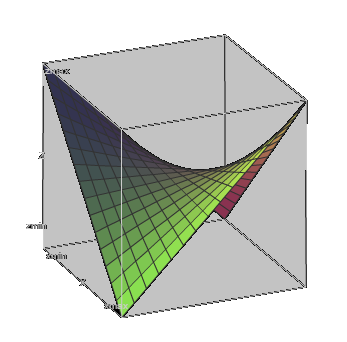
IMPORTANT NOTE The equality of partial derivatives to zero at some point is only a necessary condition for a function to have a local maximum or minimum at that point. It's not a sufficient condition. This is similar to a situation with functions of one variable, when a derivative can be zero at some point, but a function can have an inflection point like function y=x³ at point x=0. For a function of two variables a situation like this might occur when it has a saddle point. Here is an example: At the point in the middle of this "saddle" both partial derivatives are equal to zero, but this point is not a local minimum or maximum of a function.
Obviously, we would like to differentiate cases of a stationary point being a local maximum, a local minimum or a saddle point similarly to a situation with functions of one argument, where the second derivative sign (positive or negative) indicated whether a stationary point is minimum, maximum or inflection point.
Here is the rule, which we provide without rigorous proof. Let's assume that function f(x,y) can be partially differentiated twice (that is, ∂f(x,y)/∂x, ∂f(x,y)/∂y, ∂²f(x,y)/∂x², ∂²f(x,y)/∂y², ∂²f(x,y)/∂x∂y exist) and all second partial derivatives are continuous. Let's further assume that at point (a,b) both first partial derivatives equal to zero: ∂f(x,y)/∂x = 0 at x=a, y=b ∂f(x,y)/∂y = 0 at x=a, y=b Consider the expression Δ = ∂²f(x,y)/∂x² · ∂²f(x,y)/∂y² − [∂²f(x,y)/∂x∂y]² at point x=a, y=b. The rule is: if Δ < 0, (a,b) is a saddle point; if Δ > 0, (a,b) is a local minimum or local maximum point and the sign of ∂²f(x,y)/∂x² or ∂²f(x,y)/∂y² can be used to distinguish minimum from maximum (positive for minimum, negative for maximum and these two second derivatives must have the same sign since otherwise Δ would be negative). All other cases are not sufficient to determine the behavior of the function at this point.
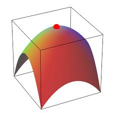
Example 1
f(x,y)=1/(1+x²+y²) ∂f(x,y)/∂x = −2x/(1+x²+y²)² ∂f(x,y)/∂y = −2y/(1+x²+y²)² At point (0,0) both partial derivatives are equal to zero, therefore (0,0) is a stationary point. Examine the second derivatives. ∂²f(x,y)/∂x² = (6x²−2y²−2)/(1+x²+y²)³ ∂²f(x,y)/∂y² = (6y²−2x²−2)/(1+x²+y²)³ ∂²f(x,y)/∂x∂y = 8x·y/(1+x²+y²)³ At point x=0, y=0 the three expressions above can be used to calculate Δ = (−2)·(−2)−0² = 4 Since Δ is positive, we have a local minimum or maximum at point (0,0). To distinguish between them, look at the sign of the second partial derivative by x. It is negative. Therefore, we have a local maximum as is obvious from the graph above.
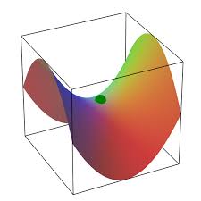
Example 2
f(x,y)=x·y ∂f(x,y)/∂x = y ∂f(x,y)/∂y = x At point (0,0) both partial derivatives are equal to zero, therefore (0,0) is a stationary point. Examine the second derivatives. ∂²f(x,y)/∂x² = 0 ∂²f(x,y)/∂y² = 0 ∂²f(x,y)/∂x∂y = 1 At point x=0, y=0 the three expressions above can be used to calculate Δ = 0·0−1² = −1 Since Δ is negative, we have a local saddle point (0,0), as is obvious from the graph above.