Induced Variable EMF: UNIZOR.COM - Physics4Teens - Electromagnetism - La...

Notes to a video lecture on http://www.unizor.com



Induced Variable EMF



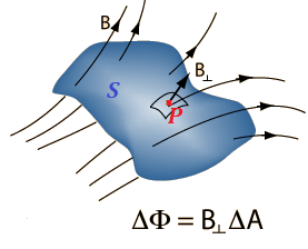
The most important fact about electromagnetic induction is that variable magnetic flux Φ(t) going through some wire frame generates in it an electromotive force (EMF) U(t) proportional to a rate of change of the magnetic flux and oppositely directed.

U(t) = −dΦ(t)/dt



Let's apply it to the following experiment.





The experiment consists of a permanent magnet moving into a wire loop,
as shown on the above picture, with different positions of a wire loop
relatively to a magnet at different times marked as t=1, t=2 etc.

At t=1 a magnet is still outside of the area of a wire loop, facing a loop with its North pole.

At t=2 a North pole of a magnet enters the area of a wire loop.

At t=3 a magnet covered half of its way through a wire loop, so the loop is positioned around a midpoint of a magnet.

At t=4 a South pole of a magnet leaves the area of a wire loop.

At t=5 a magnet is completely out of the area of a wire loop.



While the magnet is far from a wire loop (even before time t=1), practically no electricity can be observed in a wire loop. There are two reasons for it.

Firstly, the magnetic field is weak on a large distance.

Secondly, the direction of magnetic field lines in an area where a
wire loop is located at a large distance from a magnet is practically
parallel to the movement of a magnet (or movement of a wire loop
relative to a magnet). In this position a wire crosses hardly any
magnetic field lines and, consequently, the magnetic flux going through a wire loop is almost constant. Hence, the rate of the magnetic flux change is almost zero and no EMF is induced.



As we move the magnet closer (time t=1), its magnetic field in the area of a loop is increasing in magnitude and the angle between the magnetic field lines in the area of a wire loop and the direction of a wire loop relative to a magnet becomes more and more perpendicular. The magnetic flux going through a wire loop is increasing and, consequently, the EMF induced in a wire becomes more noticeable.



At time t=2 the magnitude of the magnetic field reaches
its maximum, the direction of magnetic field lines crossed by a wire
loop is close to perpendicular to a relative movement of a wire. The
magnetic flux changes rapidly and induced EMF in the wire is strong.



At time t=3 the wire loop is at the midpoint of a magnet.
The strength of a magnetic field at this position is very weak, magnetic
field lines are practically parallel to the relative movement of a
wire, and no noticeable EMF is generated.



At time t=4 the situation is analogous to that of t=2
with only difference in the direction of the magnetic field lines. Now
the wire is crossing them in the opposite direction, which causes the
induced EMF to have a different sign than at time t=2.



After that, at time t=5 the induced EMF is diminishing in magnitude and becomes almost not noticeable.



In the next experiment we replace the permanent magnet with a wire loop A
with direct current running through it. As we stated many times, the
properties of a wire loop with direct electric current going through it
are similar to those of a permanent magnet.



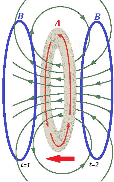
So, if we move the wire loop A with the direct current closer and closer to a wire loop B not connected to any source of electricity, the magnetic flux going through a wire loop B will be changing and, similarly to the first experiment, the induced EMF will be observed in this wire loop B.



Two positions of the loop B relative to a wire loop A are pictured above at times t=1, when wire loop A is very close to wire loop B, and t=2, when wire loop A has passed the location of wire loop B.



Similar considerations lead us to conclude that at times t=1 and t=2 the rate of change of magnetic flux through wire loop B will be the greatest and, consequently, the induced EMF in it will be the greatest.



However, these two EMF's will be opposite in direction because the
direction of crossing the magnetic lines will be opposite - at time t=1 magnetic lines are directed from inside wire loop B, but at t=2 the lines are directed into inside loop B.



In both experiments above the most important is that variable magnetic
flux going through a wire loop, not connected to any source of
electricity, induces the EMF in it.



Our third and final experiment is set as the second, except, instead of using constant direct current in the wire loop A and moving it through wire loop B to cause changing magnetic flux, we will keep the wire loop A
stationary, but will change the intensity of its magnetic field by
changing the magnitude of the electric current going through it.



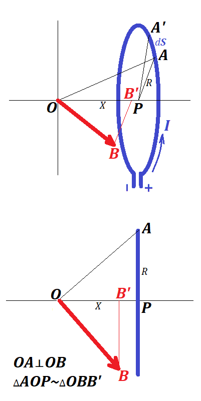
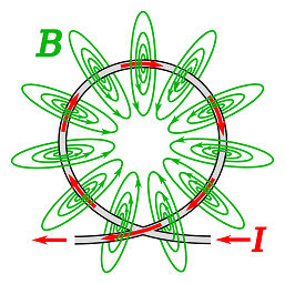
The result of changing electric current I(t) going through wire loop A of radius R (as a function of time t) is changing magnetic field vector B(t) it produces.

We did calculate the value of the intensity of this field in the center of a loop as

B(t) = μ₀·I(t)/(2R)



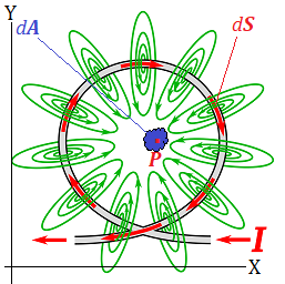
If electric current I(t) is variable, magnetic field intensity vector B(t) is variable at all points around wire loop A, including points around wire loop B, if it's relatively close.

Therefore, the magnetic flux Φ(t) through wire loop B will be variable.

Consequently, the induced EMF

U(t) = −dΦ(t)/dt

will not be zero.



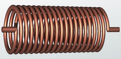
At this point it's appropriate to mention that, if wire loop A is a tight wire spiral of N loops, the variable magnetic field and, therefore, variable magnetic flux through wire loop B will be N times stronger.

That results in N times stronger EMF induced in wire loop B.



Analogously, if wire loop B is a tight wire spiral of M loops, the same EMF will be induced in each loop and, therefore, combined EMF will be M times stronger than if B consists of only a single loop.



The above considerations bring us to an idea of a transformer - a device allowing to change voltage in a circuit. This will be discussed in a separate lecture.

Solenoid: UNIZOR.COM - Physics4Teens - Electromagnetism - Magnetism of E...

Notes to a video lecture on http://www.unizor.com



Solenoid



Solenoid is a wire spiral like on this picture



It can be considered as a combination of individual circular wire loops.

We will consider an ideal case when the wire is infinitesimally thin,
the length of a solenoid along its axis is infinite and there is a
direct electric current running through it, that is running through each
of its loops.

Our purpose, as in a case of a single loop, is to determine the magnetic field inside such a solenoid.



Position our infinite in length solenoid along the X-axis such that the
X-axis is the axis of a solenoid. Let the radius of a solenoid's loops
be R and the density of the loops per unit of length along X-axis be N, that is, each, however small, segment dX on the X-axis contains N·dX loops.

Assume a direct electric current I is running through all loops.



Since a solenoid is infinite, magnetic field created by an electric
current running through it should be the same at any point on its axis.

So, let's calculate the intensity of a magnetic field B at the origin of coordinates. At any other point on the X-axis it will be the same.



The method of calculation the magnetic field is as follows.

Firstly, we will calculate the intensity of the magnetic field at
the origin of coordinates, generated by a single loop at the distance X from this point.

Secondary, we will take into account the density of the loops and
increase the calculated intensity of a single loop by a number of loops
on a segment from X to X+dX, assuming dX is infinitesimal increment.

The final step is to integrate the obtained intensity for all X from −∞ to +∞.



1. Magnetic field from a single loop at distance X from the origin of coordinates



Calculations of the magnetic field at any point on the axis going
through a wire loop is similar to but more complex than the calculation
of the magnetic field at the center of a loop we studied in the previous
lecture.

The picture below represents the general view of the wire loop with a point O,
where we want to evaluate its magnetic field and, below this general
view, the same loop as viewed from a plane this loop belongs to
perpendicularly to the X-axis.



As we know, the intensity OB of the magnetic field at point O, generated by an infinitesimal segment dS of a wire loop located at point on a loop A is perpendicular to both electric current I at point A and vector AO from a point on a loop A to a point of interest - the origin of coordinates O.



The direction of the electric current at point A is perpendicular to the plane of a picture. Therefore, vector of intensity OB is within a plane of a picture, as well as line AO. Now all lines we are interested in are on the plane of a picture and vector of magnetic field intensity OB at point of interest - the origin of coordinates O is perpendicular to a line from point A on a loop to a point of interest O:

AO⊥OB.



Let B' be a projection of the endpoint of vector OB onto X-axis. From perpendicularity of AO to OB follows that ∠AOP=∠OBB' and triangles ΔAOP and ΔOBB' are similar.



As we know, the magnitude of magnetic field intensity at point O
depends on the distance from the loop segment with electric current,
the length of this segment, the magnitude of the electric current in it
and a sine of the angle between the direction of an electric current in a
segment and the line from a segment to a point of interest:



Since the direction of the electric current is perpendicular to a plane
of a picture, the angle between the direction of an electric current in a
segment and the line from a segment to a point of interest is 90°, so
its sine is equal to 1, and the formula for intensity of a magnetic
field at point O produced by a segment dS at point A on the loop is

dB = μ₀·I·dS / [4π(R²+X²]



We should take into consideration only the X-component of the vector of
magnetic field intensity because the Y-component will be canceled by the
corresponding Y-component of a vector of intensity produced by a
segment of a loop at diametrically opposite to point A location.

Let k = sin(∠OBB').

Hence,

k = sin(∠AOP) = R/√X²+R².

Then the X-component of vector OB is

dB_x = μ₀·I·dS·k / [4π(R²+X²)] =

= μ₀·I·dS·R / [4π(R²+X²)^3/2]



To get a magnitude of the magnetic field intensity at point O from an entire loop we have to integrate the above expression by S from 0 to 2πR, and the result will be

B_x= μ₀·I·2πR² / [4π(R²+X²)^3/2]

Simplifying this gives

B(X) = μ₀·I·R² / [2(R²+X²)^3/2]

Incidentally, if our loop is located at X=0, the formula above gives

B_x = μ₀·I / (2R),

that corresponds to the results presented in the previous lecture for intensity of a magnetic field at the center of a loop.



2. Magnetic field from all loops located at distance from X to X+dX from the origin of coordinates



This is a simple multiplication of the above expression for B_x by the number of loops located at distance from X to X+dX from the origin of coordinates, which is N·dX, where N is a density of the loops in a solenoid.

The result is the intensity of a magnetic field at point O produced by an infinitesimal segment of our infinitely long solenoid from X to X+dX
μ₀·I·R²·N·dX / [2(R²+X²)^3/2]



3. Finding the magnetic field at any point inside a solenoid by integrating the intensity produced by its segment from X to X+dX by X for an entire length of a solenoid from −∞ to +∞



The above expression should be integrated by X from −∞ to +∞ to get a total value of the intensity of the magnetic field produced by an entire infinitely long solenoid at point O (or any other point on its axis).

B = γ·∫_{[−∞;+∞]} dX / (R²+X²)^3/2

where

γ = μ₀·I·N·R²/2



Substitute X=x·R in the integral with dX=R·dx.

Infinite limits for X will be infinite limits for x.

Then integral will be

∫_{[−∞;+∞]} R·dx / (R²+R²·x²)^3/2 =

= (1/R²)·∫_{[−∞;+∞]} dx / (1+x²)^3/2

The value of the integral can be easily calculated.

The indefinite integral is

x/√1+x² + C

So, the value of the definite integral between infinite limits is equal to

1 − (−1) = 2.



Therefore,

B = γ·2/R² = μ₀·I·N



IMPORTANT: The intensity of a magnetic field at any point on an axis of
an infinitely long solenoid does not depend on its radius.

Textbooks usually state that the intensity calculated above is the same
at all points inside an infinitely long solenoid, not only at the points
along its axis. The justification and the proof of this are beyond the
scope of this course.

Magnetic Flux: UNIZOR.COM - Physics4Teens - Electromagnetism - Magnetism...

Notes to a video lecture on http://www.unizor.com



Magnetic Flux



Consider a flat lying completely within an XY-coordinate plane closed
wire loop that includes a battery with direct electric current I running through it.



Since electric current generates a magnetic field around each however small segment of a wire dS
with circular magnetic field lines around it in the plane perpendicular
to this segment of a wire, the general direction of all magnetic lines
inside a wire loop will be parallel to Z-axis.

More precisely, vectors of magnetic field intensity B at
all points of XY-plane inside a wire loop are similarly directed
perpendicularly to this plane and parallel to Z-axis. They are not
necessarily equal in magnitude, though.



Consider an infinitesimal two-dimensional area of XY-plane inside a wire loop dA around some point P.
Since it's infinitesimal, we can assume that the intensity of the
magnetic field inside it is uniform and equal to the intensity at point P, which we will denote as vector B(P).

This intensity is a result of combined magnetic field generated at that point by all infinitesimal segments dS of a wire.

Each one of these components of a resulting intensity vector has a
direction perpendicular to a direction of electric current in segment dS (its source) and to a vector R from a chosen infinitesimal segment dS of a wire loop to point P, from which follows the perpendicularity of all vectors of magnetic field intensity to XY-plane and parallel to Z-axis.



Magnetic field, as other force fields, is additive, that is, the
combined intensity vector generated by an entire wire loop is a vector
sum of intensity vectors generated by each segment of a wire.



All these individual magnetic fields generated by different segments of a
wire are directed along the Z-axis, so we will concentrate only on
their magnitude to find the result of their addition.



Knowing the geometry of a wire and the electric current I in it, we can use the law we described in the previous lecture that determines the magnetic field intensity at any point P inside a wire loop generated by its any infinitesimal segment dS:

dB = μ₀·I·dS·sin(α) / (4πR²)

where

R is a magnitude of a vector R from a chosen infinitesimal segment dS of a wire loop to point P,

dS is the infinitesimal segment of a wire,

α is an angle between the direction of electric current in the segment dS and a vector R from this segment to a point P,

μ₀ is the permeability of free space.



Integrating this along the entire wire (this is integration along a curve) gives the value of magnetic field intensity B(P) at point P.



Now we assume that this process is done and function B(P) is determined, that is we know the magnitude B(P) of the intensity vector of magnetic field generated by our wire loop at any point P inside a loop.

Recall that the direction of this vector is always along Z-axis, that is perpendicular to a plane of a wire loop.



We define magnetic field flux Φ as a two-dimensional integral of a product of intensity B(P) by area dA.

In a simple case of a constant magnetic field intensity B(P)=B at any point P inside a loop this is a simple product of a constant magnetic field intensity B by the area of a wire loop A

Φ = B · A

If B(P) is variable inside a loop, the two-dimensional integration by area of the loop produces the magnetic field flux

Φ = ∫∫_AB(P)·dA



The complexity of exact calculation of magnetic field intensity B(P) at any point P inside a loop and subsequent calculation of the magnetic field flux
flowing through the wire loop are beyond the scope of this course, so
in our practice problems we will usually assume the uniformity of the
magnetic field with constant B(P)=B.



A concept of magnetic field flux is applicable not only for a
magnetic field generated by a wire loop with electric current running
through it. It is a general concept used to characterize the combined
effect of a magnetic field onto the area where we observe it.



Consider an analogy:

magnetic field intensity and amount of grass growing in the backyard in a season per unit of area,

wire loop area and area of a backyard,

magnetic field flux and how much grass growth in an entire backyard in a season.

Another analogy:

magnetic field intensity and productivity of each individual doing some work,

wire loop area and a team of people doing this work,

magnetic field flux and productivity of a team doing this work.



A general magnetic field flux is defined for a given magnetic field with known intensity vector B(P) at each point P of space and given two-dimensional finite surface S in space, through which magnetic field lines are going.



The purpose of our definition of magnetic field flux in this general case is to quantify the total amount of "magnetic field energy" flowing through a surface S.



Notice a small area around point P on a picture above.

If we consider it to be infinitesimally small, we can assume that
magnetic field intensity at any point of this small area is the same as
at point P.



If this small area is perpendicular to vector B(P), we would just multiply the magnitude of intensity vector B(P) in tesla by the area ΔA of a small area around point P in square meters and obtain the magnetic field flux ΔΦ going through this small area in units of magnetic flux -
weber = tesla · meter².

In a more general case, when this small area around point P is not perpendicular to magnetic field intensity vector B(P), to obtain the magnetic field flux going through it, we have to multiply it by cos(φ), where φ(P) is an angle between magnetic field intensity vector B(P) and normal (perpendicular vector) to a surface at point P.

So, the expression for an infinitesimal magnetic field flux around point P is

dΦ = B(P)·cos(φ(P))·dA



The unit of measurement of magnetic field flux is Weber (Wb) that is equal to a flux of a magnetic field of intensity through an area of

1 tesla (1T)1 square meter (1m²):

1 Wb = 1 T · 1 m²



Once we have determined the magnetic field flux flowing through a
small area around each point of a surface, we just have to summarize
all these individual amounts to obtain the total magnetic field flux flowing through an entire surface.

Mathematically, it means we have to integrate the above expression for dΦ along a surface S.



We will not consider this most general case in this course. Our magnetic fields will be, mostly, uniform and surfaces flat.

Problems on Self-Induction: UNIZOR.COM - Physics4Teens - Electromagnetis...

Notes to a video lecture on http://www.unizor.com



Problems on Self-Induction



Problem A



Consider a wire of resistance R₀ bent into a circle of a radius r with its ends connected to a battery producing a voltage U₀.

There is a switch that can turn the flow of electricity in this circuit ON or OFF during a short time period T.

When it turns ON, the resistance of the circuit, as a function of time R(t), changes from infinitely large value to the value of R₀ as

R(t) = R₀·T/t

When it turns OFF, the resistance changes from the value of R₀ to an infinitely large value as

R(t) = R₀·T/(T−t)

What is the EMF of self-induction U_i during the current switching ON or OFF?



Solution



Switching ON

According to the Ohm's Law, the electric current in the circuit is

I(t) = U₀ /R(t) = U₀·t /(R₀·T)

The magnetic field intensity inside a loop, as we discussed in the lecture on magnetism of a current in a loop, is

B(t) = μ₀·I(t) /(2r) = μ₀·U₀·t /(2r·R₀·T)

The magnetic flux going through the wire loop of the radius r is a product of the intensity of the magnetic field by the area of a loop

Φ(t) = B(t)·πr² = μ₀·U₀·t·πr² /(2r·R₀·T) = πμ₀·U₀·t·r /(2R₀·T)

The EMF of self-induction is the first derivative of the magnetic flux
by time with a minus sign (minus sign because the induced EMF works to
prevent the increase in the current)

U_i = −dΦ/dt = −πμ₀·U₀·r /(2R₀·T)

It's negative, so it reduces the overall voltage in the circuit and,
therefore, reduces the electric current in it. At the end of switching
ON (at t=T) the current will not reach its maximum value but will continue to rise after the switch is completely ON until it reaches it.



Switching OFF

According to the Ohm's Law, the electric current in the circuit is

I(t) = U₀ /R(t) = U₀·(T−t) /(R₀·T)

The magnetic field intensity inside a loop, as we discussed in the lecture on magnetism of a current in a loop, is

B(t) = μ₀·I(t) /(2r) = μ₀·U₀·(T−t) /(2r·R₀·T)

The magnetic flux going through the wire loop of the radius r is a product of the intensity of the magnetic field by the area of a loop

Φ(t) = B(t)·πr² = μ₀·U₀·(T−t)·πr² /(2r·R₀·T) = πμ₀·U₀·(T−t)·r /(2R₀·T)

The EMF of self-induction is the first derivative of the magnetic flux
by time with a minus sign (minus sign because the induced EMF works to
prevent the increase in the current)

U_i = −dΦ/dt = πμ₀·U₀·r /(2R₀·T)

It's positive, so it adds to the overall voltage in the circuit and,
therefore, increases the electric current in it, which, potentially, can
be harmful for electronic devices on the circuit.





Problem B



In the same setting as in Problem A calculate minimum time T_min of switching a circuit OFF in order for the current in a circuit grow no more then 10% from the theoretical value

I₀ = U₀ /R₀,I₀ = U₀ /R₀.



Solution



Induced EMF equals to (from Problem A)

U_i = πμ₀·U₀·r /(2R₀·T)

It's a constant and does not depend on time t.

The resistance of a circuit is growing with time from R₀ at t=0 to infinity at t=T. Therefore, the maximum electric current will be observed at t=0, when the resistance is minimal, and will equal to

I_max = (U₀+U_i) /R₀ = I₀ + (U_i /R₀)

In order for this current not to exceed I₀ by 10% the following inequality must be satisfied

U_i /R₀ ≤ 0.1·U₀ /R₀

The resistance cancels and the remaining inequality is

U_i ≤ 0.1·U₀

Using the value of U_i calculated in Problem A, we obtain the following inequality that should be resolved for time interval T

πμ₀·U₀·r /(2R₀·T) ≤ 0.1·U₀

Voltage U₀ cancels out and the remaining inequality for time interval T is

T ≥ πμ₀·r /(0.2R₀)



Practical case

Assume the following conditions

μ₀ = 4π·10⁻⁷ N/A²

r = 0.1 m

R₀ = 200 Ω

Then the time interval of switching OFF must be at least

T = πμ₀·r /(0.2R₀) ≅ 10⁻⁸ sec

That is a very short interval of time. Mechanical switches usually are
much slower, which means the electric current under normal usage in
homes will not significantly rise when we switch the electricity OFF.

IMPORTANT:

Check formula units

(N/A²)·m/Ω = N·m/(A²·Ω) =

[N·m → W → V·A·sec]

= (V·A·sec)/(A²·Ω) =

[Ω → V/A]

= (V·A·sec·A)/(A²·V) = sec

as it is supposed to be.

Self-Induction: UNIZOR.COM - Physics4Teens - Electromagnetism -

Notes to a video lecture on http://www.unizor.com



Self-Induction



Let's study the process of increasing the direct electric current in a
wire loop that is connected to a source of a direct electricity (like
battery) that generates electromotive force of voltage U₀.

This increase might be attributed to a decrease in resistance in this
loop. For example, if the wire loop was initially disconnected from a
source of electricity and we connected it, flipping some switch, the
resistance is changing from being practically infinite to some value R during a fraction of a second and the electric current would grow from zero to some value

I = U/R (Ohm's Law).





The first thing that we can observe is that there is a magnetic field
generated by an electric current with magnetic field lines going through
a loop, thus effectively making it a magnet.



The next thing we note is that the intensity of a magnetic field
generated by an increasing direct current is also increasing with the
current because of their relationship that we have described in the
lecture about magnetism of an electric current loop.

In the center of an ideally circular loop this intensity, as we calculated in that lecture, is

B = μ₀·I/(2R)

where

μ₀ is permeability of space,

I is the current in a wire loop,

R is the radius of a wire loop.



At other points around the wire the intensity of a magnetic field also
increases proportionally to the electric current in a wire. Even if the
shape of our wire loop is not ideally circular, the proportionality of
intensity of a magnetic field at any point to an electric current would
still be held, because each infinitesimal segment of a wire creates its
own magnetic field and the magnetic field intensity is an additive
function, that is, produced by two sources, intensities from each are
added as vectors, resulting in a combined intensity.

As a result, the magnetic flux going through a wire loop increases proportionally to an increase in electric current.



Now recall the Faraday's Law of magnetic induction. It states that changing magnetic flux going through an electric circuit generates electromotive force (EMF) proportional to a rate of change of the magnetic flux, where rate of change means a change per unit of time, which, using mathematical language, is the first derivative of a variable magnetic flux by time.



Let's ignore for now the signs of the rate of change of the magnetic flux and the EMF, then the Faraday's Law can be represented as

U = dΦ/dt

where

U is the absolute value of a magnitude of the generated EMF,

Φ is magnetic flux,

t is time,

dΦ/dt is the rate of change of magnetic flux (first derivative of magnetic flux by time), taken as an absolute positive value.



From

(1) the proportionality of a magnetic field intensity at any point around a wire to an electric current going through a wire,

(2) definition of magnetic flux and

(3) the Faraday's Law

follows that the increasing electric current, causing an increasing
magnetic flux going through a circuit (so, the first derivative of a
magnetic flux is positive), generates a secondary EMF in
the circuit that is proportional to a rate of change of a magnetic flux,
which, in turn, is proportional to a rate of change of the electric
current in a loop.

So, generated (induced) secondary EMF is proportional to a rate of change of an electric current in a loop.



This induced secondary EMF causes the secondary electric current in a loop that interferes with the original electric current.

The process of interference of two electric currents, varying original
one and that caused by a change of magnetic field flux, is called self-induction.



Now let's talk about the direction of that secondary current from the position of the Law of Energy Conservation.

If the secondary current flows in the same direction as the increasing
original one, the rate of change of electric current in a loop will
increase, causing a greater rate of change of the magnetic flux, causing
even greater rate of change of the electric current flowing through a
wire, causing even greater flux etc. This is a perfect source of free
energy, so it cannot be true.

Indeed, the secondary electric current must be directed opposite to an
increasing original one, thus slowing the rate of increase.

The EMF generated by self-induction is opposite to the one that originated the increase in the electric current in a loop.



As a practical implication of this principle, when we switch a lamp on,
and the time a switch actually closes the circuit is, for example 0.01
sec, the electric current in a circuit will not reach its maximum during
this exact time, but later, like during 0.02 sec, because of
self-induction that slows the increase of amperage.



Let's consider the process of decreasing of the electric current in a
loop, like when we disconnect a wire from a primary source of
electricity.



Decreasing electric current in a wire loop causes proportional decrease
of a magnetic field intensity at any point around a wire.

This, in turn, causes proportional decrease of magnetic flux flowing through a wire loop with rate of change (first derivative of flux by time) negative.

Negative rate of change of magnetic flux causes the generation of secondary (induced) EMF in a wire, that results in a secondary electric current, that interferes with the decreasing primary one.



Let's analyze the direction of this secondary electric current.

Above, when the primary electric current was increasing and the rate of change of magnetic flux was positive,
we concluded that induced EMF causes the secondary electric current to
go in the opposite to primary direction to preserve the Law of Energy
Conservation.



In a case of decreasing primary electric current we see that the
magnetic flux flowing through a wire loop is decreasing, it's rate of
change (first derivative) is negative, so the secondary (induced) EMF must be directed opposite to the one generated by an increasing primary electric current.



Therefore, if in the case of increasing primary electric current the secondary EMF "worked" against the electric current,
generating a secondary current in a direction opposite to an increasing
primary one, in the case of decreasing primary current the secondary (induced) EMF generates the secondary current in the same direction as a decreasing primary current, "helping" the decreasing primary current, prolonging the decrease.



So, in both cases the secondary (induced) EMF works opposite to a rate of change of the magnetic flux going through a wire loop.

When the magnetic flux increases, the induced EMF generates an
electric current in the opposite direction to a primary one, thus
slowing the rate of increase of the electric current and, therefore,
against the rate of increase of the magnetic flux.

When the magnetic flux decreases, the induced EMF generates an
electric current in the same direction as a primary one, thus slowing
the decrease of the electric current and, therefore, against the rate of
decrease of the magnetic flux.



The above considerations are the primary reason why the Faraday's Law is expressed as
U = −dΦ/dt

where the minus sign signifies that the induced EMF works against the rate of change of a magnetic flux.

Current in a Loop: UNIZOR.COM - Physics4Teens - Electromagnetism - Magne...

Notes to a video lecture on http://www.unizor.com



Magnetism of Electric Current in a Loop



Let's recall some general considerations of any field produced by a
point-source (like gravitational or electrostatic) and the force it
exerts at certain distance from its center.



In three-dimensional space the field influence is spreading around in
all directions from its center, and at any given time it reaches and
spreads over a sphere of the area 4πR², where R is the radius of this sphere.



This important consideration prompted the dependency between the
magnitude of the field force at any point in space and inverse of a
square of a distance between this point and the source of a field.

This dependency exists in all laws related to fields we studied, and it's true for magnetic field as well.



There is, however, an important complication with the sources of
magnetic field. Strictly speaking, they are not and theoretically cannot
be just points, because they always have a characteristic of the
direction. If it's a permanent magnet, there is a North pole to South
pole direction. If the source is a direct current, there is a direction
of electrons that causes the existence of a magnetic field.

So, besides the distance from the source of a magnetic field, another
important aspect that influences the magnetic field is how the point of
measuring the magnetic field is positioned relatively to a direction of
the electric current at the source of a field.



Consider measuring a strength of a magnetic field at point P on the following picture.



Here an infinitesimal segment AB of the length dS of a wire with an electric current I produces a magnetic field that we are measuring at point P. From the viewpoint of point P segment AB is visible at an angle and seems having the size of a segment BC that is perpendicular to a radius-vector R from the source of magnetic field segment AB to the point of measuring P.



Simple geometry gives the visible from point P length of segment AB - the length of BC, which is the length of AB multiplied by sin(α).



With this correction to a simple dependency of the strength of magnetic
field on the inverse square of a distance from the field source we can
represent the magnitude of the vector of magnetic field strength or
intensity at point P as

dB = k·I·dS·sin(α) / R²

The constant k in SI units equals to μ₀/(4π), where μ₀ is the permeability of free space. So the formula for a magnitude of the strength of magnetic field looks like this:

dB = μ₀·I·dS·sin(α) / (4πR²)



The vector of force has magnitude and direction. The magnitude was
evaluated above. The direction of this force, based on experimental
data, is always perpendicular to both the direction of the current I and the direction of the radius-vector from the source of magnetic field to a point of measurement P.



This allows us to express the vector of magnetic field intensity B in a form of a vector product

B = μ₀·I·dS ⨯ r / (4πR²)

where r is a unit vector in the direction from the source of magnetic field segment AB to the point of measurement P.

Equivalent formula is

B = μ₀·I·dS ⨯ R / (4πR³)



Let's apply this formula to calculate the magnetic field intensity and direction in a center of a circular wire loop of radius R with electric current I running through it.



We divide the circular wire loop into infinitesimal segments of the length dS. Fortunately, all radiuses from any such segment to a center of a loop are perpendicular to these segments, so sin(α)=1 in the above formula for a magnitude of the intensity vector.



The magnetic field intensity B from each segment equals to

dB = μ₀·I·dS / (4πR²)

The direction of this force is perpendicular to both radius to a segment dS
and to a segment itself. That is, it should be perpendicular to a plane
of the wire loop, that is the vector of magnetic field force in a
center of a wire loop is always directed perpendicularly to the loop.

Since it's true for any segment dS, we can just add all the forces from all the segments, that is, we have to integrate the above expression by S along the whole circle from 0 to 2πR.

The only variable in the above expression is dS, so the result is

B = ∫_[0,2πR] μ₀·I·dS/(4πR²) =

= 2πR·μ₀·I/(4πR²)= μ₀·I/(2R)

UNIZOR.COM - Physics4Teens - Electromagnetism

Notes to a video lecture on http://www.unizor.com



Problems on
Electromagnetic Induction



Problem A



The following experiment is conducted in the space with Cartesian coordinates.

Two infinitely long parallel wires in XY-plane are parallel to X-axis, one at Y-coordinate y=a and another at Y-coordinate y=−a (assuming a is positive).

These two wires are connected by a third wire positioned along the Y-coordinate between points (0,a) and (0,−a).

The fourth wire, parallel to the third one, also connects the first two,
but slides along the X-axis, always maintaining its parallel position
to Y-axis. The X-coordinate of its position is monotonously increasing
with time t according to some rule x=x(t).

All four wires are made of the same material and the same cross-section with the electrical resistance of a unit length r.



There is a uniform magnetic field of intensity B with field lines parallel to Z-axis.

Initial position of the fourth wire coincides with the third one, that is x(0)=0.



What should the function x(t) be to assure the generation of the same constant electric current I₀ in the wire loop?

What is the speed of the fourth rod at initial time t=0?



Solution



The area of a wire frame is changing with time:

S(t)=2a·x(t).

Magnetic flux through this wire frame is

Φ(t)=B·S(t).

Therefore, the magnitude of the generated electromotive force or voltage U(t), as a function of time, is

U(t) = dΦ(t)/dt = 2B·a·x'(t)

The resistance R(t) of the wire loop, as a function of time, is a product of a resistance of a unit length of a wire r by the total length of all four sides of a wire rectangle L=4a+2x(t).

R(t) = r·L = 2r·[2a+x(t)]

The electric current I(t) in a wire loop, according to the Ohm's Law, is

I(t) = U(t)/R(t) =

= 2B·a·x'(t) / {2r·[2a+x(t)]} =

= B·a·x'(t) / {r·[2a+x(t)]}

This current has to be constant and equal to I₀. This leads us to a differential equation I₀=I(t)

I₀ = B·a·x'(t) / {r·[2a+x(t)]}

Simplifying this equation, obtain

I₀·r / (B·a) = x'(t) / [2a+x(t)]

[I₀·r / (B·a)]·dt =

= d[2a+x(t)] / [2a+x(t)]

Integrating,

[I₀·r / (B·a)]·t + C = ln(2a+x(t))

2a + x(t) = C·e^{I₀·r·t / (B·a)}

Since x(0)=0, C=2a

x(t) = 2a·[e^{I₀·r·t / (B·a)} − 1]

Speed of the motion of the fourth wire along the X-axis is

x'(t) = 2a·e^{I₀·r·t/(B·a)}·[I₀·r/(B·a)]

or

x'(t) = e^{I₀·r·t/(B·a)}·[2I₀·r/B]

At time t=0 the initial speed is

x'(0) = 2I₀·r / B





Problem B



A rectangular wire frame in a space with Cartesian coordinates rotates with variable angular speed ω(t) in a uniform magnetic field B.

In the beginning at t=0 the wire frame is at rest, ω(0)=0.
As the time passes, the angular speed is monotonously increasing from
initial value of zero to some maximum. This models turning the rotation
on.

The axis of rotation is Z-axis.

The initial position of a wire frame is that its plane coincides with XZ-plane.



The magnetic field lines are parallel to X-axis.

So the angle between the magnetic field lines and the wire frame plane φ(t) at t=0 equals to zero.

The sides of a wire frame parallel to Z-axis (those, that cross the magnetic field lines) have length a, the other two sides have length b.



Determine the generated electromotive force (EMF) in this wire frame as a function of time t.


Solution



The angle φ(t) between the magnetic field lines and the
wire frame plane is changing with time. In the initial position, when
the wire frame coincides with XZ-plane, this angle is 0°, since magnetic
field lines are stretched along the X-axis.

As the wire frame rotates with variable angular speed ω(t), the angle between magnetic field lines and the wire frame plane φ(t) and the angular speed ω(t) are related as follows

dφ/dt = φ'(t) = ω(t)



This is sufficient to determine the value of φ(t) by integration of the angular speed on a time interval [0,t]

φ(t) = ∫_[0,t] ω(τ)·dτ



Magnetic field flux Φ(t) flowing through a wire frame depends on the intensity of the magnetic field B, area of a wire frame S=a·b and angle φ(t) the plane of a wire frame makes with magnetic field lines.

Φ(t) = B·S·sin(φ(t))



The electromotive force (voltage) U(t) generated by rotating wire frame equals to a rate of change (first derivative) of the magnetic field flux

U(t) = dΦ(t)/dt =

= B·S·cos(φ(t))·φ'(t) =

= B·S·cos(φ(t))·ω(t)

where angle φ(t) can be obtained by an integration of an angular speed presented above.