Viscosity Damping 1
Over-Damping
Another variety of damping is related to viscosity of the environment, where oscillation takes place.
An example of this is an oscillation under water.
Each motion of an object on a spring in this case is supposed to overcome a resistance of water that surrounds it.
Interesting distinction of an oscillation under water from previously studied oscillation with friction is that the resistance of water is greater if the speed of an oscillating object is greater, while the friction resistance is constant and depends only on the weight of an object.
This property of the force of resistance to be dependent on (for our theoretical studies to be proportional to) speed is expressed by a formula that is supported by experiments:
Fv(t) = −c·x'(t)
where
t is time parameter;
Fv(t) is the force of resistance caused by viscosity of the environment where oscillation occurs;
x(t) is a displacement of an object from the neutral position on a spring (positive displacement corresponds to stretching, negative - to squeezing a spring);
x'(t) is an object's speed (first derivative of displacement);
c is a damping coefficient that depends on geometrical properties of an object and physical properties of environment, where oscillation takes place.
A minus sign in the formula signifies that the resistance force is opposite to a direction of movement, defined by a sign of a speed.
Equipped by the formula above and by Hooke's Law, describing the force of a spring on an object Fs(t) as being proportional to a displacement of an object from its neutral position on a spring x(t) with coefficient of proportionality k that depends on elasticity of a spring
Fs(t) = −k·x(t)
we come up with a total force Ft(t) acting on an object, oscillating in a viscous environment:
Ft(t) = Fs(t) + Fv(t)
Since the object's acceleration (second derivative of displacement) x"(t) and mass m are related to the total force acting on an object by the Second Newton's Law
Ft(t) = m·x"(t)
we have an equation of motion for an oscillating object in the viscous environment
m·x"(t) = −k·x(t) − c·x'(t)
or
m·x"(t) + c·x'(t) + k·x(t) = 0
This is linear differential equation that we will solve to get the formula for a displacement of an object from its neutral position on a spring x(t) as a function of time.
At this point we'd like to refer you to "Math 4 Teens" course on the same site UNIZOR.COM as this lecture will help to refresh your knowledge about linear differential equations of the second order. From the Unizor home screen choose "Math 4 Teens" - "Calculus" - "Ordinary Differential Equations, Higher Order Equations", where Hooke's Law is presented and general approach to solving linear differential equations of the second order is discussed.
The general solution to a linear differential equation of the second order, like the one above, can be found by finding two functions that satisfy this equation x1(t) and x2(t), called partial solutions, and describing the general solution as a linear combination of these two functions
x(t) = A·x1(t) + B·x2(t).
The coefficients A and B depend on two initial conditions x(0) and x'(0).
In the lecture about Hooke's Law, as an example of linear differential equation of the second order, it was suggested to seek partial solutions based on function x(t) = eγ·t
where γ - some (generally, complex) number.
The reason for this is that, substituting this function with its first and second derivatives into the differential equation, we get
x'(t) = γ·eγ·t
x"(t) = γ²·eγ·t
and the differential equation is
γ²·m·eγ·t + γ·c·eγ·t + k·eγ·t = 0
Canceling eγ·t, which never equal to zero, we get a quadratic equation for γ
γ²·m + γ·c + k = 0
with any of its solutions (generally, complex), used in function eγ·t, delivering the solution of the original differential equation.
Since a quadratic equation has exactly two solutions among complex numbers γ1 and γ2, we have two solutions to our original differential equations: x1(t)=eγ1·t and x2(t)=eγ2·t.
Moreover, since the differential equation is linear, any linear combination of the above two solutions will be a solution to a differential equation.
Therefore, the general solution looks like
x(t) = A·eγ1·t + B·eγ2·t
where constants A and B are defined by two initial conditions of the motion described by our differential equation.
Switching from theory to concrete results for our differential equation presented above, our first task is to solve the quadratic equation to find γ1 and γ2
γ²·m + γ·c + k = 0
Very important for a solution to this equation is an expression under radical - discriminant Δ=c²−4k·m.
If it's not negative, both roots of our equation are real, otherwise we have to consider complex roots.
Solutions to this equations are:
γ1,2 = [−c±√c²−4k·m] /(2m)
or
γ1,2 = −c/(2m)±√(c/(2m))²−k/m
At this point we will consider three different cases of a discriminant of our quadratic equation:
Δ=c²−4k·m is positive
Δ=c²−4k·m equals to zero
Δ=c²−4k·m is negative
The first case is analyzed in this lecture, two others - in the next.
Case 1
Δ=c²−4k·m is POSITIVE
Let
ω² = Δ /m² = (c/(2m))²−k/m
where ω - some non-negative real number.
Obviously, ω is smaller then c/(2m).
Then the solutions to our equations are
γ1,2 = −c/(2m) ± ω
Since ω is smaller then c/(2m), both solutions to our quadratic equation are negative.
General solution to our differential equation is
x(t) = A·e(−c/(2m)+ω)·t +
+ B·e(−c/(2m)−ω)·t
Let's determine coefficients A and B from initial conditions on the position and speed of an object.
At t=0 the position is x(0)=a and speed is x'(0)=0.
From this follows
A + B = a
(−c/(2m)+ω)·A +
+ (−c/(2m)−ω)·B = 0 Simplifying the second equation, we get the system of 2 linear equations with two unknowns A and B
A + B = a
−c/(2m)·(A+B) + ω·(A−B) = 0 Using the first equation for A+B=a in the second one, we obtain:
A + B = a
−c·a/(2m) + ω·(A−B) = 0
or A + B = a
A − B = c·a/(2m·ω)
From these two equations we obtain the values of A and B:
A = a·[1+c/(2m·ω)]/2
B = a·[1−c/(2m·ω)]/2
Solution to our differential equation with given initial conditions is
x(t) = (a/2)·[1+c/(2m·ω)]·
·e(−c/(2m)+ω)·t +
+ (a/2)·[1−c/(2m·ω)]·
·e(−c/(2m)−ω)·t
This function describes the position of an object on a spring at any moment of time t relatively to its neutral position on a spring.
Regardless of the signs of coefficients A and B, both exponents in the above expression for x(t) are negative and each term is monotonously going to zero as time t increases to infinity, so the whole function x(t) that characterizes the displacement of the object on a spring in a viscous environment is decreasing to zero as time t increases to infinity. That is, the object moves towards its neutral position on a spring.
To further investigate the character of object's movement, let's find its speed, as it moves toward the neutral position. It requires to take the derivative of the above function describing its position.
x'(t) = (a/2)·(−c/(2m)+ω)·
·[1+c/(2m·ω)]·e(−c/(2m)+ω)·t +
+ (a/2)·(−c/(2m)−ω)·
·[1−c/(2m·ω)]·e(−c/(2m)−ω)·t =
= (a/2)·e−c·t/(2m)·
·[(ω−c²/(4ωm²))·eωt +
+ (−ω+c²/(4ωm²))·e−ωt] =
= (a/(8ωm²))·e−c·t/(2m)·
·[(4ω²m²−c²)·eωt +
+ (−4ω²m²+c²)·e−ωt] =
= (a/(8ωm²))·e−c·t/(2m)·
·(−4m·k·eωt+4m·k·e−ωt) =
= (a·k/(2ωm))·e−c·t/(2m)·
·(−eωt+e−ωt)
The expression for x'(t) can only be equal to zero, if eωt=e−ωt,
which possible only if t=0.
Notice that, since ω is a non-negative real number smaller then c/(2m), the absolute value of x'(t) is decreasing to zero as time goes to infinity.
This means that the object's speed never equals to zero after initial moment, our object never stops, never changes the direction and monotonously moves towards its neutral position on a spring, moving slower and slower, as it comes closer to the neutral position.
Let's calculate the exact expression for this function for some sample values of the constants involved:
a=12
m=1
c=10
k=16
Δ=c²−4m·k=36
ω²=(c/(2m))²−k/m=9
ω=3
−c/(2m)+ω=−2
−c/(2m)−ω=−8
A=a·[1+c/(2m·ω)]/2=16
B=a·[1−c/(2m·ω)]/2=−4
x(t) = 16·e−2t−4·e−8t
Now let's check if this solution satisfies our differential equation
m·x"(t) + c·x'(t) + k·x(t) = 0
Substituting the assumed values for coefficients, it looks like this:
x"(t) + 10·x'(t) + 16·x(t) = 0
Let's check it out for our sample function
x(t) = 16·e−2t−4·e−8t
x'(t) = −32·e−2t+32·e−8t
x"(t) = 64·e−2t−256·e−8t
Substituting these expressions into equation
x"(t) + 10·x'(t) + 16·x(t) =
= 64·e−2t−256·e−8t −
−320·e−2t+320·e−8t +
+ 256·e−2t−64·e−8t =
= (64−320+256)·e−2t+
+ (−256+320−64)·e−8t =
= 0 (OK)
Let's check the initial conditions.
x(0)=16−4=12=a (OK)
x'(0)=−32+32=0 (OK)
Let's draw a graph of our sample function
x(t) = 16·e−2t−4·e−8t
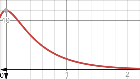
This graph confirms that the displacement of an object from the neutral position monotonically goes to zero, that is it moves in one direction only towards the neutral position without oscillation.
The effect of damping of viscous environment is so strong that it prevents the object to oscillate on a spring.
This is called over-damping or large damping.

No comments:
Post a Comment